Insurance Fraud Detection with Graph Analytics

Author(s): Tony Zhang

Originally published on Towards AI the World’s Leading AI and Technology News and Media Company. If you are building an AI-related product or service, we invite you to consider becoming an AI sponsor. At Towards AI, we help scale AI and technology startups. Let us help you unleash your technology to the masses.

Explore graph database and extract graph features to augment the machine learning model

Insurance fraud is an enormous problem, and the insurance industry has been fighting fraud for a very long time. Let’s see the following headline new and statistics:

Insurance fraud costs U.S. consumers at least $80 billion every year, according to The Coalition Against Insurance Fraud (CAIF). CAIF also estimates that workers’ compensation insurance fraud alone costs insurers and employers $30 billion a year. The FBI reports that non-health insurance portion of the overall problem amounts to $40 billion annually. Ultimately, the massive scope of the problem can mean the average U.S. family will pay an extra $400 and $700 per year in premiums.

Health insurance fraud is a type of white-collar activity wherein dishonest claims are filed to gain a profit. The fraudulent activity may involve peers of providers, physicians, and beneficiaries acting together to make fraud claims. Hence, it is difficult to detect fraudulent activities given the complexity of the parties involved. The anomalous behavior could be a fraud ring where providers, doctors, and clients file small claims over time. Such small claims can be difficult to detect with traditional tools, which look at the claims individually and cannot uncover the connections between the various players.

A graph database is designed to fill the gap by storing and handling the highly connected data where the relationship is as important as the individual data point. Hence, we can utilize graph analytics to understand the relationships. In this article, you will learn :

• Graph basic
• Graph search and query to understand the relationships
• Augment machine learning model with graph features

Graph basic

What is graph?

In mathematics, and more specifically in graph theory, a graph is a structure amounting to a set of objects in which some pairs of the objects are in some sense “related”. The objects correspond to mathematical abstractions called vertices (also called nodes or points) and each of the related pairs of vertices is called an edge (also called link or line).

Simply put, a graph is a mathematical representation of any type of network with:

• Vertex, sometimes called a node, in the insurance context, can be:
  – Claim
  – Policyholder
• Edge is the relationship/interaction/behavior between the nodes:
  – Policyholder of claim
  – Insured of claim

Graph algorithm concepts will be introduced in the third chapter — Augment machine learning model with graph features.

Graph search and query

Graph database is purpose-built to store and navigate the relationships utilizing the connectivity between vertices. End users don’t need to execute countless joins as the graph query language is about pattern matching between nodes. This is more natural to work with and can be easily used by business users whose feedback can be fed into the fraud detection system.

Graph visualization through the graph query language helps to analyze a large amount of data and identify patterns that indicate fraudulent activities. In this section, I will share a few scenarios, and the visualizations are based on:

• Source of data: Analyzing insurance claims using IBM Db2 graph
• Graph database: Nebula Graph

Fraud signal warning

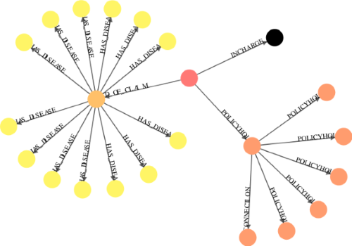
Find all claims filed by the policyholder of fraudulent claim “C4377” and show the diseases of claim “C4377” patient.

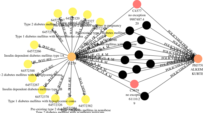
To deep dive into this policyholder(PH3759), we see that this person saw different doctors at different providers, which is not normal.

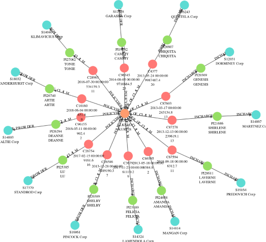
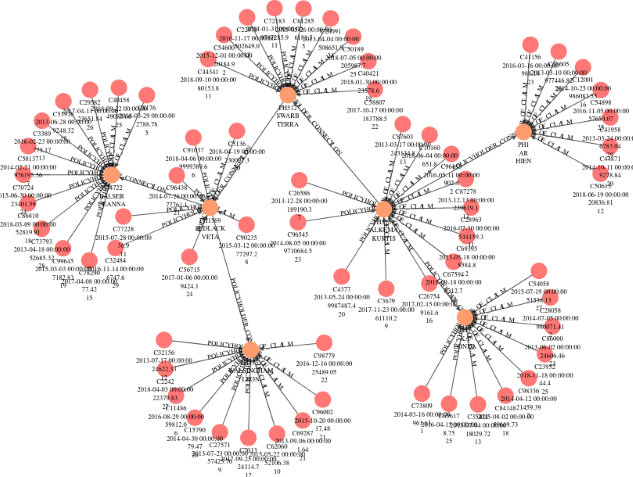
Policyholder connections related to the fraudulent claim

The graph shows the connections of the high-risk profile that has the fraud claim “C4377”. We see one high-risk policyholder in the 1st-degree connection and another high-risk policyholder in the 3rd-degree connection.

Augment machine learning model with graph features

Feature engineering is the art of formulating useful features from existing data. The definition is:

Feature engineering is the process of transforming raw data into features that better represent the underlying problem to the predictive models, resulting in improved model accuracy on unseen data.

Many machine learning applications typically rely on tabular data models and omit the relationship & contextual data, which are the strongest predictors of behavior. This is crucial as each individual claim/provider may look legitimate by avoiding red flags.

In this section, I will walk through a concrete example of how to transform the tabular data into a graph and extract graph features to augment the machine learning model. The overall approach is:

• Ingest tabular data into graph structure in Python
• Feature engineering on the graph data
• Incorporate graph features into the machine learning pipeline

Caveats:

• we are predicting whether a claim is fraudulent or not based on the provider’s fraudulent flag
• the idea is to show the process of creating potential predictive features and augment the current machine learning pipeline

Ingest Tabular Data into Graph Structure

In this section, I will use:

• Source of data: HEALTHCARE PROVIDER FRAUD DETECTION ANALYSIS
• Python graph package: iGraph

The dataset is from Medicare and consists of claims filed by the providers as well as information about the beneficiary for every claim:

• Patient-related features: age, gender, location, health conditions, etc.
• Claim-related features: start & end date, claim amount, diagnosis code, procedure code, provider, attending physician, operating physician, etc.

Nodes in this article are providers and attending physicians who are source and target, respectively.

# import package
from igraph import *

# use time-based split to avoid data leakage
Train_Inpatient_G = Train_Inpatient[Train_Inpatient['ClaimStartDt'] < '2009-10-01'][['Provider', 'AttendingPhysician', 'ClaimID']].reset_index(drop = True)
Train_Outpatient_G = Train_Outpatient[Train_Outpatient['ClaimStartDt'] < '2009-10-01'][['Provider', 'AttendingPhysician', 'ClaimID']].reset_index(drop = True)

# merge inpatient and outpatient data
G_df = pd.concat([Train_Inpatient_G, Train_Outpatient_G], ignore_index = True, sort = False)
G_df.shape

# implement edge with weight
G_df = G_df[['Provider', 'AttendingPhysician', 'ClaimID']]
G_df = G_df.groupby(['Provider', 'AttendingPhysician']).size().to_frame('Weight').reset_index()
G_df.shape

source = 'Provider'
target = 'AttendingPhysician'
weight = 'Weight'

G_df[source] = G_df[source].astype(str)
G_df[target] = G_df[target].astype(str)
G_df.shape

# create graph from dataframe
G = Graph.DataFrame(G_df, directed=False)

Feature engineering on graph data

Using graph algorithms, I create new potential meaningful features, such as connectivity metrics and clustering features based on the relationship. In order to prevent target leakage, I use the time-based split to generate graph features. In this section, I will provide code for graph features:

Degree

The node can be defined as the number of edges incident to a node.

degree = pd.DataFrame({'Node': G.vs["name"],
        'Degree': G.strength(weights = G.es['Weight'])})
degree.shape

Closeness

In a connected graph, closeness centrality (or closeness) of a node is a measure of centrality in a network, calculated as the reciprocal of the sum of the length of the shortest paths between the node and all other nodes in the graph.

closeness = pd.DataFrame({'Node': G.vs["name"],
        'Closeness': G.closeness(weights = G.es['Weight'])})
closeness.shape

Infomap

Infomap is a graph clustering algorithm capable of achieving high-quality communities.

communities_infomap = pd.DataFrame({'Node': G.vs["name"],
        'communities_infomap': G.community_infomap(edge_weights = G.es['Weight']).membership})
communities_infomap.shape

The resulting metrics from the graph algorithms are transformed into a table so that the generated features can be used in a machine learning model.

# merge graph features
graph_feature = [degree, closeness, eigenvector_centrality, pagerank, communities_infomap, community_multilevel]
graph_feature = reduce(lambda left,right: pd.merge(left,right, how = 'left',on='Node'), graph_feature)

Incorporate graph features into the machine learning pipeline

The graph features are merged into the raw model-ready data, and the time-based split is utilized to prepare the data for the machine learning model.

train = Final_Dataset_Train[Final_Dataset_Train['ClaimStartDt'] < '2009-10-01'].reset_index(drop = True).drop('ClaimStartDt', axis = 1)
print(train.shape)
test = Final_Dataset_Train[Final_Dataset_Train['ClaimStartDt'] >= '2009-10-01'].reset_index(drop = True).drop('ClaimStartDt', axis = 1)
print(test.shape)

x_tr = train.drop(axis=1,columns=['PotentialFraud'])
y_tr = train['PotentialFraud']

x_val = test.drop(axis=1,columns=['PotentialFraud'])
y_val = test['PotentialFraud']

In this article, I explored 6 scenarios with the combination of 2 algorithms and 3 feature spaces:

• Algorithm:
  – Logistic Regression
  – Random Forest
• Feature space:
  – original features
  – original features + node level features
  – original features + node level features + clustering features

lr = LogisticRegression(penalty='none', solver='saga', random_state=42, n_jobs=-1)
rf = RandomForestClassifier(n_estimators=300, max_depth=5, min_samples_leaf=50, 
                            max_features=0.3, random_state=42, n_jobs=-1)
lr.fit(x_tr, y_tr)
rf.fit(x_tr, y_tr)
preds_lr = lr.predict_proba(x_val)[:,1]
preds_rf = rf.predict_proba(x_val)[:,1]

Here I use AUC as the evaluation metric on the test set and the ROC curve is below:

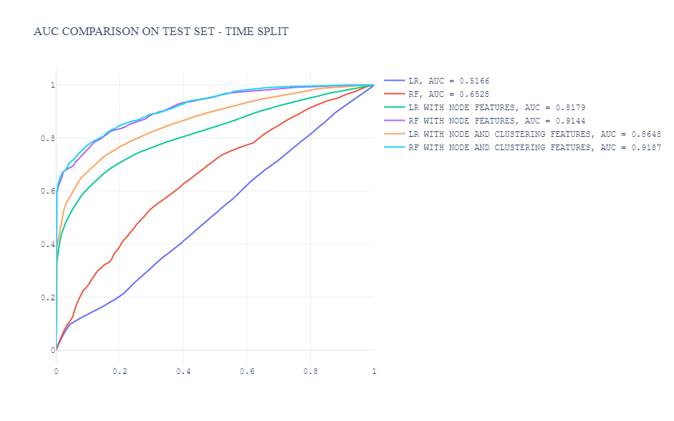
Generally, as the plot above, we can summarize:

• Outperformance by the model with graph features
• Outperformance by Random Forest with node level and clustering features

In this article, I didn’t dive deep into model interpretation and model diagnosis. Earlier, I wrote an article on model interpretation — Deep Learning Model Interpretation Using SHAP, which you may be interested in.

Conclusion

• A graph database can be queried, visualized, and analyzed by business users to discover fraud schemes, especially for the fraudulent activities that try to hide through complex network structures, which could be quite a difficult task in a conventional data structure.
• Incorporating relationship information and adding these potential predictive features into the current machine learning pipeline can improve model performance, especially for scenarios in that multiple parties are involved in fraudulent activities.

Reference

https://www.iii.org/article/background-on-insurance-fraud

https://en.wikipedia.org/wiki/Graph_(discrete_mathematics)

https://github.com/IBM/analyzing-insurance-claims-using-ibm-db2-graph

https://github.com/vesoft-inc/nebula

https://machinelearningmastery.com/discover-feature-engineering-how-to-engineer-features-and-how-to-get-good-at-it/

https://www.kaggle.com/datasets/rohitrox/healthcare-provider-fraud-detection-analysis

https://igraph.org/python/

https://en.wikipedia.org/wiki/Degree_(graph_theory)

https://en.wikipedia.org/wiki/Closeness_centrality

https://towardsdatascience.com/deep-learning-model-interpretation-using-shap-a21786e91d16

---

Insurance Fraud Detection with Graph Analytics was originally published in Towards AI on Medium, where people are continuing the conversation by highlighting and responding to this story.

Join thousands of data leaders on the AI newsletter. It’s free, we don’t spam, and we never share your email address. Keep up to date with the latest work in AI. From research to projects and ideas. If you are building an AI startup, an AI-related product, or a service, we invite you to consider becoming a sponsor.

Published via Towards AI