


How Should We Detect and Treat the Outliers?
Last Updated on October 18, 2022 by Editorial Team
Author(s): Gowtham S R
Originally published on Towards AI the World’s Leading AI and Technology News and Media Company. If you are building an AI-related product or service, we invite you to consider becoming an AI sponsor. At Towards AI, we help scale AI and technology startups. Let us help you unleash your technology to the masses.
What are outliers? How do we need to detect outliers? How do we need to treat the outliers?
Table of Contents:
· What are Outliers?
· Outlier Detection and Removal Techniques:
· Z Score-based method
· IQR technique
· Percentile Method
What are Outliers?
An outlier is that datapoint or observation which behaves very differently from the rest of the data.
If we are finding the average net worth of a group of people, and if we find Elon Musk in that group, then the complete analysis will go wrong because of just one outlier. This is a reason why outliers should be treated properly before building a machine learning model.
Simple ways to write Complex Patterns in Python in just 4mins.
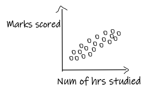
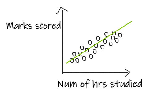
If we are building a linear regression model, which has an independent feature, ‘Num of hours studied’, and the dependent feature, ‘marks scored’, and if the data is distributed as shown below, then the model will perform well.
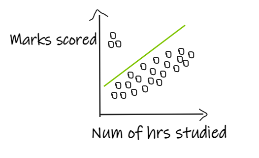
If we have 3 students who scored good marks even after studying for fewer hours, then the regression line shifts in order to fit the outlier points as shown below, resulting in giving bad results to the actual data.
Machine learning algorithms in which the calculation of weight is involved, like linear regression, logistic regression, Ada boost, and deep learning models, will get impacted by the outliers. Tree-based algorithms like Decision trees, Random Forest will get less impacted by outliers.
How do I Verify the Assumptions of Linear Regression?
In anomaly detection algorithms like insurance fraud detection or credit card fraud detection, we need to catch the outliers, in this kind of situation, the purpose is to catch the outliers.
So we need to treat the outliers carefully,
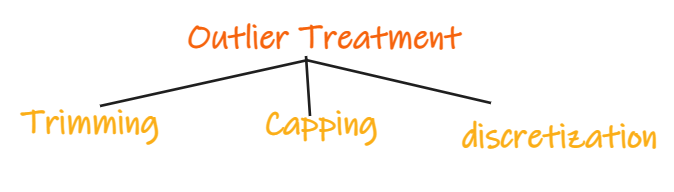
Trimming: Remove the outliers from the dataset before training a machine learning model. E.g., Remove the students from the dataset in the above example.
Capping: Keep a maximum or minimum threshold and give values to the data points accordingly. E.g., if we are working on the age feature, we can keep the threshold of 85 and assign the value of 85 to all the people with age greater than 85.
Discretization: This is the method in which numerical features are converted to discrete using bins. E.g., if the age 80–90 is considered as a single bin, then all the ages between 80 and 90 will be treated equally.
Outlier Detection and Removal Techniques:
1. Z Score-based method
The main assumption in this technique is that the data should be normally distributed or close to normal distribution.
If the data is normally distributed, the Empirical Rule says that 68.2% of the data points lie in between the 1st standard deviation, 95.4% of the data points lie in between the 2nd standard deviation, and 99.7% of the data points will be between the 3rd standard deviation.
Data points that lie outside the 3rd standard deviation can be treated as outliers.
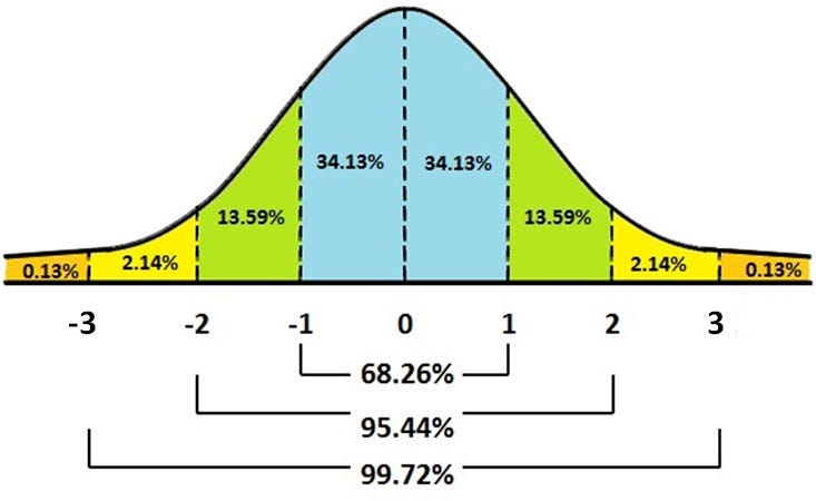
As 99.7% of the data will lie within the 3 standard deviations, we can treat the rest of the data which lie outside the 3 standard deviations as outliers.
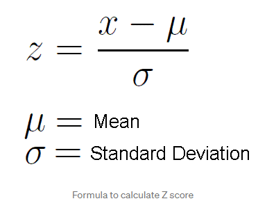
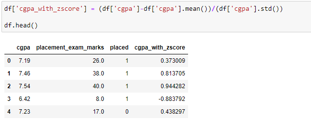
Standardization or Z-Score Normalization is one of the feature scaling techniques, here, the transformation of features is done by subtracting from the mean and dividing by standard deviation. This is often called Z-score normalization. The resulting data will have the mean as 0 and the standard deviation as 1.
Standardization vs Normalization
Let us look at the practical implementation of this technique.
import pandas as pd
import numpy as np
import seaborn as sns
import matplotlib.pyplot as plt
import warnings
warnings.filterwarnings('ignore')
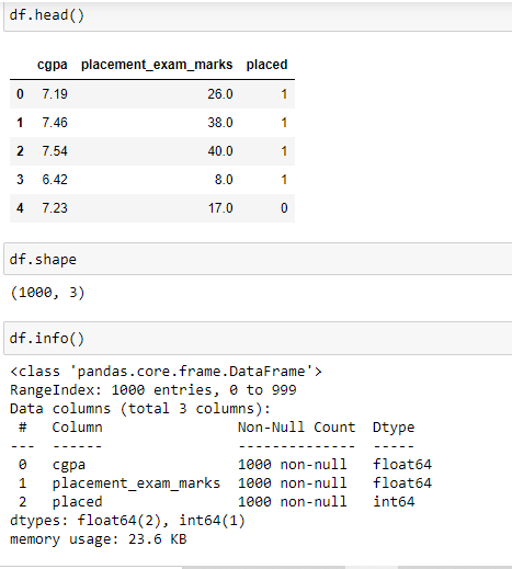
df = pd.read_csv('placement_dataset.csv')
The dataset has 2 independent features cgpa and placement_exam_marks.
plt.figure(figsize=(10,5))
plt.subplot(1,2,1)
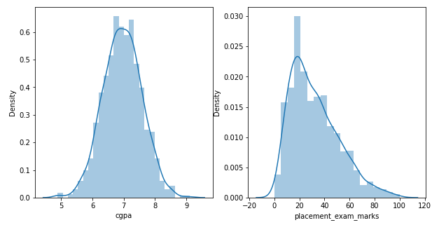
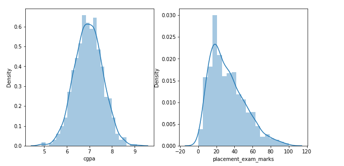
sns.distplot(df['cgpa'])
plt.subplot(1,2,2)
sns.distplot(df['placement_exam_marks'])
The distribution of the data shows that the feature cgpa is normally distributed, and the other feature, placemet_exam_marks is skewed.
So, the feature cgpa qualifies for the Z Score-based method of the outlier detection technique.
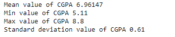
print('Mean value of CGPA {}'.format(df['cgpa'].mean()))
print('Min value of CGPA {}'.format(df['cgpa'].min()))
print('Max value of CGPA {}'.format(df['cgpa'].max()))
print('Standard deviation value of CGPA {}'.format(round(df['cgpa'].std(),2)))
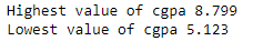
# the boundary values are:
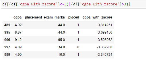
print('Highest value of cgpa', round(df['cgpa'].mean()+3*df['cgpa'].std(),3))
print('Lowest value of cgpa', round(df['cgpa'].mean()-3*df['cgpa'].std(),3))
Below are the 5 data points which are detected as outliers.
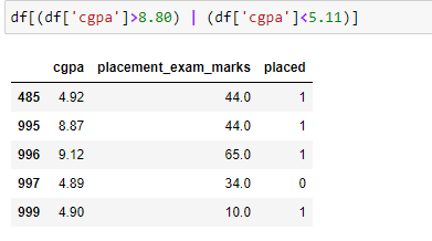
This can also be achieved using the Z score formula, which is shown below.
Outlier Treatment:
Trimming: In this method, we can remove all the data points that are outside the 3 standard deviations.
Sometimes, if the dataset has a large number of outliers, then we lose a significant amount of data.
Capping: In this method, the outlier data points are capped with the highest or lowest values, as shown below.
Why Is Multicollinearity A Problem?
2. IQR technique
This method is used when the distribution of the data is skewed.
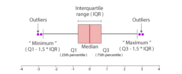
The IQR describes the middle 50% of values when ordered from lowest to highest. To find the interquartile range (IQR), first, find the median (middle value) of the lower and upper half of the data. These values are quartile 1 (Q1) and quartile 3 (Q3). The IQR is the difference between Q3 and Q1.
IQR = Q3-Q1
Minimum value = Q1–1.5 *IQR
Maximum value = Q3+1.5*IQR
The data points which are lesser than the minimum value and the data points which are greater than the maximum value are treated as outliers.
Let us look at the practical implementation of this technique.
plt.figure(figsize=(10,5))
plt.subplot(1,2,1)
sns.distplot(df['cgpa'])
plt.subplot(1,2,2)
sns.distplot(df['placement_exam_marks'])
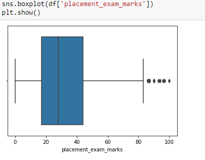
The feature placement_exam_marks is skewed and qualifies for the IQR method of outlier detection.
df['placement_exam_marks'].skew()
0.8356419499466834
#Finding the IQR
Q1 = df['placement_exam_marks'].quantile(0.25)
Q3 = df['placement_exam_marks'].quantile(0.75)
IQR = Q3-Q1
upper_limit = Q3+1.5*IQR
lower_limit = Q1-1.5*IQR
print('lower limit: ', lower_limit)
print('upper limit: ', upper_limit)
print('IQR:' , IQR)
lower limit:  -23.5
upper limit:  84.5
IQR: 27.0
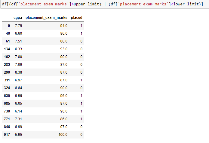
The above 15 data points are detected as outliers.
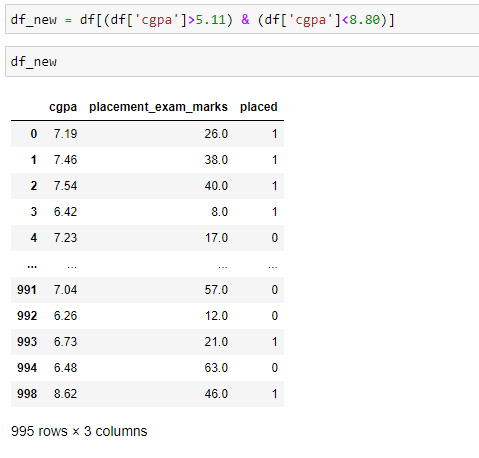
Trimming:
In this method, we can remove all the data points that are outside the minimum and maximum limits.
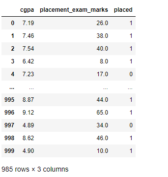
df_new = df[~(df['placement_exam_marks']>upper_limit) | (df['placement_exam_marks']<lower_limit)]
df_new
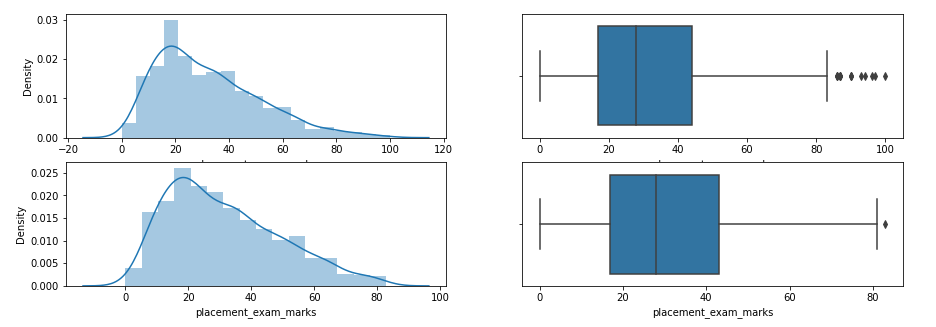
plt.figure(figsize=(15,5))
plt.subplot(2,2,1)
sns.distplot(df['placement_exam_marks'])
plt.subplot(2,2,2)
sns.boxplot(df['placement_exam_marks'])
plt.subplot(2,2,3)
sns.distplot(df_new['placement_exam_marks'])
plt.subplot(2,2,4)
sns.boxplot(df_new['placement_exam_marks'])
Look at the distribution of data and boxplot after trimming the feature.
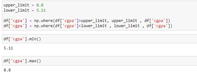
Capping:
In this method, the outlier data points are capped with the highest or lowest values, as shown below.
upper_limit = 84.5
lower_limit = -23.5
df_cap = df.copy()
df_cap['placement_exam_marks'] = np.where(df_cap['placement_exam_marks']>upper_limit, upper_limit , df_cap['placement_exam_marks'])
df_cap['placement_exam_marks'] = np.where(df_cap['placement_exam_marks']<lower_limit , lower_limit , df_cap['placement_exam_marks'])
df_cap['placement_exam_marks'].max()
84.5
df_cap['placement_exam_marks'].min()
0.0
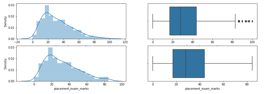
We can compare the distribution of the data before and after capping the features.
plt.figure(figsize=(15,5))
plt.subplot(2,2,1)
sns.distplot(df['placement_exam_marks'])
plt.subplot(2,2,2)
sns.boxplot(df['placement_exam_marks'])
plt.subplot(2,2,3)
sns.distplot(df_cap['placement_exam_marks'])
plt.subplot(2,2,4)
sns.boxplot(df_cap['placement_exam_marks'])
Look at the distribution of data and boxplot after capping the feature.
How do I Analyze the data before building a machine learning model?
3. Percentile Method
In simple words, Percentile can be seen as the value below which a percentage of data falls. If my score is 90 percentile, then that means my score is better than 90 percent of the students who took the examination.
If you scored the maximum score, which happens to be 95, then it is 100 percentile, which means you scored more than the 100% of the students who took the examination.
This is one of the simplest techniques used to detect the outliers in a dataset. We need to just decide the threshold, Eg, if we decide 1 percentile, then it means we treat all the values above 99 percentile and below 1 percentile as outliers.
Let us look at how we can implement this method practically.
df = pd.read_csv('weight-height.csv')
df.head()
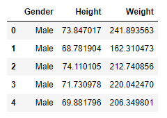
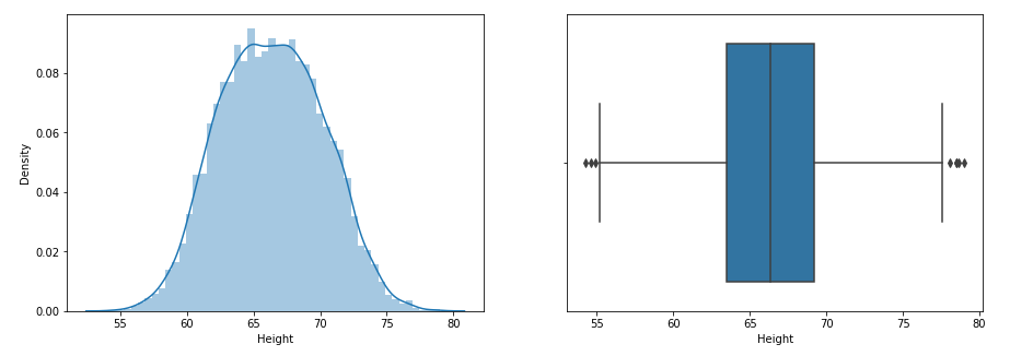
Let us apply the percentile method to the feature ‘Height’.
plt.figure(figsize=(15,5))
plt.subplot(1,2,1)
sns.distplot(df['Height'])
plt.subplot(1,2,2)
sns.boxplot(df['Height'])
Look at the distribution of data and boxplot of the feature.
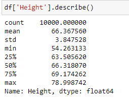
#Finding the upper and lower limit
upper_limit = df['Height'].quantile(0.99)
lower_limit = df['Height'].quantile(0.01)
print('lower limit: ', lower_limit)
print('upper limit: ', upper_limit)
lower limit:  58.13441158671655
upper limit:  74.7857900583366
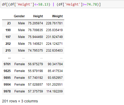
The above 201 data points are detected as outliers.
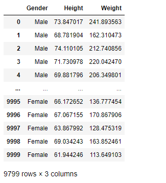
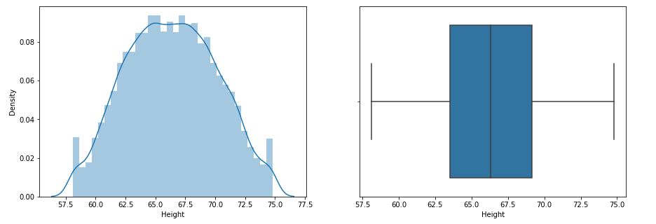
Trimming
In this method, we can remove all the data points that are outside the minimum and maximum limits.
df_new = df[(df['Height']>=58.13) & (df['Height']<=74.78)]
df_new
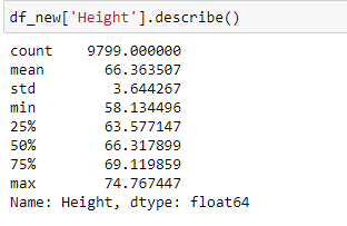
plt.figure(figsize=(15,5))
plt.subplot(1,2,1)
sns.distplot(df_new['Height'])
plt.subplot(1,2,2)
sns.boxplot(df_new['Height'])
Look at the distribution of data and boxplot after trimming the feature.
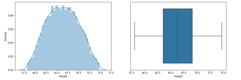
Capping (Also called Winsorization)
In this method, the outlier data points are capped with the highest or lowest values as shown below.
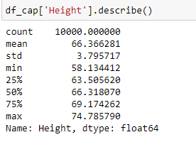
upper_limit = df['Height'].quantile(0.99)
lower_limit = df['Height'].quantile(0.01)
df_cap = df.copy()
df_cap['Height'] = np.where(df_cap['Height']>upper_limit , upper_limit , df_cap['Height'])
df_cap['Height'] = np.where(df_cap['Height']<lower_limit , lower_limit , df_cap['Height'])
plt.figure(figsize=(15,5))
plt.subplot(1,2,1)
sns.distplot(df_cap['Height'])
plt.subplot(1,2,2)
sns.boxplot(df_cap['Height'])
Look at the distribution of data and boxplot after capping the feature.
Please visit the GitHub link to get the complete code.
You can connect with me via LinkedIn
How Should We Detect and Treat the Outliers? was originally published in Towards AI on Medium, where people are continuing the conversation by highlighting and responding to this story.
Join thousands of data leaders on the AI newsletter. It’s free, we don’t spam, and we never share your email address. Keep up to date with the latest work in AI. From research to projects and ideas. If you are building an AI startup, an AI-related product, or a service, we invite you to consider becoming a sponsor.
Published via Towards AI
Towards AI Academy
We Build Enterprise-Grade AI. We'll Teach You to Master It Too.
15 engineers. 100,000+ students. Towards AI Academy teaches what actually survives production.
Start free — no commitment:
→ 6-Day Agentic AI Engineering Email Guide — one practical lesson per day
→ Agents Architecture Cheatsheet — 3 years of architecture decisions in 6 pages
Our courses:
→ AI Engineering Certification — 90+ lessons from project selection to deployed product. The most comprehensive practical LLM course out there.
→ Agent Engineering Course — Hands on with production agent architectures, memory, routing, and eval frameworks — built from real enterprise engagements.
→ AI for Work — Understand, evaluate, and apply AI for complex work tasks.
Note: Article content contains the views of the contributing authors and not Towards AI.
Related posts
Recent Posts


")


