How I built Supervised Skin Lesion Segmentation on HAM10000 Dataset

Author(s): Sriram S M

 

Originally published on Towards AI.

Skin cancer is one of the most common types of cancer in the world. Its early diagnosis is pivotal for eliminating malignant tumors from the human body.

There is a lot of ongoing research on skin cancer detection, localization, and classification. Segmentation is an essential step in the localization of skin cancer.

Segmentation is a technique used in computer vision to identify objects or boundaries to simplify an image and more efficiently analyze it.

It is performed by dividing an image into different regions based on the characteristics of pixels. Binary Segmentation is used to divide two major regions of the image. Binary Segmentation, in particular, is used in skin cancer localization.

# importing the required libraries

!pip install lightning
import lightning as pl

import numpy as np
import pandas as pd
import seaborn as sns

import os
import torch
import matplotlib.pyplot as plt
import torchvision
import torchvision.transforms as transforms
!pip install segmentation-models-pytorch
import segmentation_models_pytorch as smp
from PIL import Image
from pprint import pprint
from torch.utils.data import DataLoader

Data Set

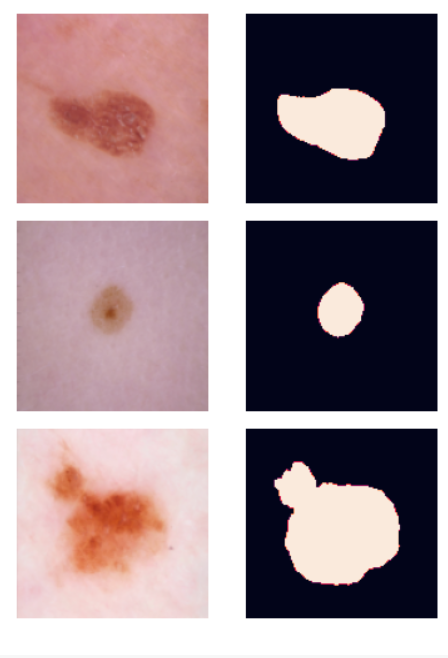
To explore Binary Segmentation, I used the popularly available HAM10000 Dataset of 10015 skin lesion images with the type of cancer and their corresponding masks.

Masks are 2D images with pixel intensities of either 1 (high) or 0 (low). They are essentially the product of any binary segmentation task, as our goal is to divide the image into two major regions.

The types of cancer in the dataset include:

• Actinic keratoses and intraepithelial carcinoma / Bowen’s disease (AKIEC),
• basal cell carcinoma (BCC),
• benign keratosis-like lesions (solar lentigines / seborrheic keratoses and lichen-planus-like keratoses, BKL),
• dermatofibroma (DF),
• melanoma (MEL),
• melanocytic nevi (NV)
• vascular lesions (angiomas, angiokeratomas, pyogenic granulomas and hemorrhage, VASC).

Some data exploration was done on the data set. It was found that the most common type of cancer was Melanocytic Nevi with a 67% share.

GT = pd.read_csv('/content/GroundTruth.csv')
gt = GT.sum().to_frame().reset_index().drop(0)
gt.columns = ['toc', 'sum']

plt.figure(figsize=(15,9))
explode = [0, 0.1, 0, 0, 0, 0, 0]
plt.pie(gt[‘sum’], labels=gt[‘toc’],explode=explode, autopct=’%.0f%%’)
plt.show()

Since my focus was on segmentation, I focused only on the images. The type of cancer could be used in other downstream tasks, such as cancer classification.

Some EDA was done on the ground truth masks. Using the fraction of pixel intensities, I found the distribution of the size of the lesion compared to the image size.

Note: A point to note here is that the zoom level of the images when they were captured is not known. Zoom level can immensely affect the analysis done here. Since we have no information about it in the data, we can revisit some outliers. This gives us an idea of whether the reason for the change in the fraction covered is severity or zoom level. Upon monitoring a few of the outliers, it was found that some images appear to be taken through a microscope, indicating a high zoom level, whereas some others appear to be taken using just a camera.

To avoid this kind of deviation in the dataset, a more structured way of data collection should be followed, such as additional meta-data on how the image was captured and under what level of zoom. This will enhance the quality of the data set and any downstream tasks performed on it.

This analysis is done under the assumption that all the images had the same zoom level or under the assumption that the zoom level does not affect our approach significantly.

lesion_fracs = []
for i in range(len(resized_masks)):
 uniques, vc = np.unique(resized_masks[i].numpy(), return_counts=True)
 if len(vc) == 1:
 lesion_fracs.append(0)
 else:
 lesion_fracs.append(vc[1]/(vc[0]+vc[1]))

lfs = pd.DataFrame(lesion_fracs)

plt.figure(figsize=(8,5))
sns.set_style(‘darkgrid’)
sns.distplot(lfs, bins = 20)
plt.title(‘Distribution of size of skin lesion’, fontdict={‘size’: 20})
plt.xlabel(‘Fraction of image covered by skin lesion’, fontdict={‘size’: 10})
plt.ylabel(‘Frequency’, fontdict={‘size’: 10})
plt.show()

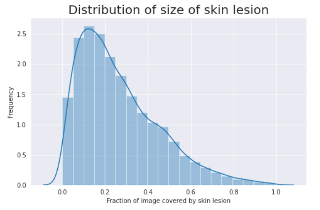
The distribution of the size of skin lesions looks skewed towards the left side, with the most frequent ‘fraction of image covered by skin lesion’ of ~10–20%. Since our model will be built based on this data, if we are to test a different data set on our model, we will have to ensure a similar distribution of lesion sizes.

Approach

A high-level idea for the approach used is as follows. The specifics and detailed descriptions are provided later on.

• Model — To perform the task of binary segmentation, a Convolution Neural Network is used.
• Input — The input to our CNN would be an RGB image from the dataset resized to 128×128.
• Output — The output would be a 2D mask image of the size 128×128.
• Loss function — Dice loss is used as the loss function for this model. It is a common metric used in binary segmentation.
• Tracking metric — Jaccard Index/Intersection over Union is another popular metric in binary segmentation.

Model

The python library ‘segmentation models pytorch’ was used to easily create and handle the CNN model. ‘segmentation models pytorch’ allows us to create a model by combining encoder and decoder architectures and pre-trained weights from popular CNN architectures like ResNet, VGGNet, UNet, etc. The model which was used for the task had:

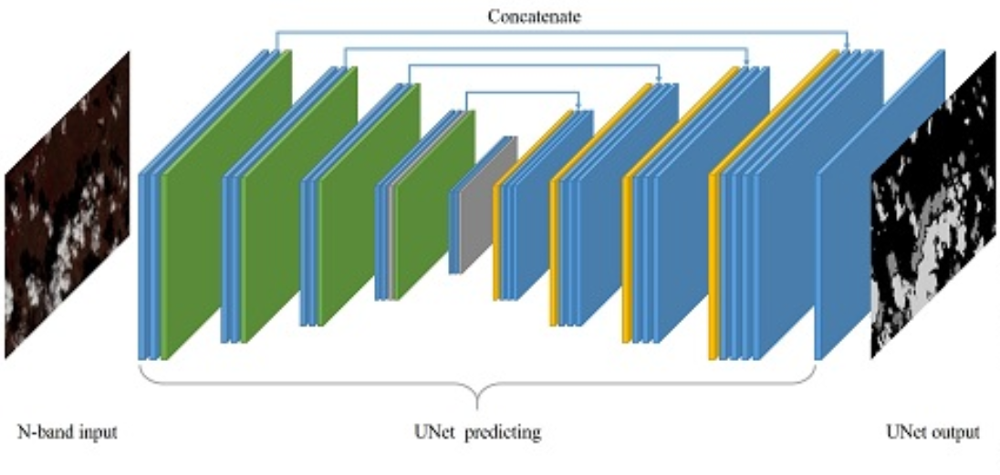
• U-net architecture: To exploit the strength of the encoder-decoder framework and skip connections from the encoder to the decoder. The encoder converts the image to a concise lower-dimensional shape by using a series of convolutional layers and max pooling layers.
  The decoder then converts the concise shape to the required output shape through a series of convolutional and upscaling layers.
  This framework is found to be effective because converting the information to a lower dimensional vector removes noise and helps better training on important features.
  The additional skip connections are found to increase the quality of the output.
• Resnet34 encoder and decoder with pre-trained weights on ImageNet: To help with good initialization. ImageNet is a popular image dataset used in competitions and for comparing models.
  By using pre-trained weights, we are ensuring the model’s ability to identify important features to start with.
  This helps us use lesser data and lesser training time since most of the work is done and only finetuning to our task is needed.

class SegmentationModel(pl.LightningModule):

def __init__(self, arch, encoder_name, in_channels, out_classes, **kwargs):
super().__init__()
self.model = smp.create_model(
arch, encoder_name=encoder_name, in_channels=in_channels, classes=out_classes, **kwargs
)

# preprocessing parameteres for image
params = smp.encoders.get_preprocessing_params(encoder_name)
self.register_buffer(“std”, torch.tensor(params[“std”]).view(1, 3, 1, 1))
self.register_buffer(“mean”, torch.tensor(params[“mean”]).view(1, 3, 1, 1))

# dice loss as loss function for binary image segmentation
self.loss_fn = smp.losses.DiceLoss(mode=’binary’, from_logits=True)

def forward(self, image):
image = (image – self.mean) / self.std
mask = self.model(image)
return mask

def _step(self, batch, stage):

image = batch[0] # Shape of the image : (batch_size, num_channels, height, width)
mask = batch[1]

logits_mask = self.forward(image)
loss = self.loss_fn(logits_mask, mask)

prob_mask = logits_mask.sigmoid()
pred_mask = (prob_mask > 0.5).float()

tp, fp, fn, tn = smp.metrics.get_stats(pred_mask.long(), mask.long(), mode=”binary”)
return {“loss”: loss, “tp”: tp, “fp”: fp, “fn”: fn, “tn”: tn,}

def _epoch_end(self, outputs, stage):

tp = torch.cat([x[“tp”] for x in outputs])
fp = torch.cat([x[“fp”] for x in outputs])
fn = torch.cat([x[“fn”] for x in outputs])
tn = torch.cat([x[“tn”] for x in outputs])

# micro-imagewise – first calculate IoU score for each image and then compute mean over these scores
per_image_iou = smp.metrics.iou_score(tp, fp, fn, tn, reduction=”micro-imagewise”)

metrics = {
f”{stage}_per_image_iou”: per_image_iou,
}

self.log_dict(metrics, prog_bar=True)

def training_step(self, batch, batch_idx):
return self._step(batch, “train”)

def training_epoch_end(self, outputs):
return self._epoch_end(outputs, “train”)

def validation_step(self, batch, batch_idx):
return self._step(batch, “valid”)

def validation_epoch_end(self, outputs):
return self._epoch_end(outputs, “valid”)

def test_step(self, batch, batch_idx):
return self._step(batch, “test”)

def test_epoch_end(self, outputs):
return self._epoch_end(outputs, “test”)

def configure_optimizers(self):
return torch.optim.Adam(self.parameters(), lr=0.0001)

model = SegmentationModel(“Unet”, “resnet34”, in_channels=3, out_classes=1)

Input and Output

The images in the data set were of shape (3,450,600), indicating that they are color images with 3 channels — RGB, and have a height of 450 pixels and width of 600 pixels. These images were resized to (3,128,128).

This is because the encoder-decoder architecture of CNNs easily handles sizes of power of 2. Higher-quality images are computationally expensive, but down-sampling too much will result in the loss of important features.

So 128 was chosen to balance the trade-off between image quality and computational time. The 2D output masks and the ground truth masks too, were set to the same size (128,128).

# The following transforms were used on the images

transform = transforms.Compose([
transforms.Resize((128, 128)),
transforms.ToTensor(),
])

resized_images = []
for image in images[:4000]:
resized_image = transform(image)
resized_images.append(resized_image)

resized_masks = []
for mask in masks[:]:
resized_mask = transform(mask)
if resized_mask.squeeze()[0][0]*resized_mask.squeeze()[0][-1]*resized_mask.squeeze()[-1][0]*resized_mask.squeeze()[-1][-1] == 1:
resized_mask = -resized_mask.round()+1
resized_masks.append(resized_mask.round())

Loss function and metrics

The quality of results from a machine learning model is highly influenced by what metric we use to evaluate and assess the model. Different evaluation metrics and loss functions can be used to test our model performance.

In any prediction task, for every data point, we have a ground truth which is the expected correct output, and a corresponding prediction that the model outputs. The purpose of an evaluation metric is to give us an idea of how close the prediction is to the ground truth.

Now that we have a qualitative intuition behind what the purpose of a metric is, we use the prediction and ground truth to make up a quantitative formula. Let us suppose a classification task of 2 output 2 classes. So for every data point, the output can be either of the 2 classes, say 0 (Negative class) and 1 (Positive class).

Now for every data point, we have a corresponding ground truth and a prediction. We can split the dataset into 4 parts:

• True Positives (TP): The data points where both ground truth and prediction were class 1.
• True Negatives (TN): The data points where both ground truth and prediction were class 0.
• False Positives (FP): The data points where ground truth was class 0 and prediction was class 1.
• False Negatives (FN): The data points where ground truth was class 1 and the prediction was class 0.

By looking at these measures we see that we would aim to maximize TP and TN and minimize FP and FN.

’Accuracy’ is a well-known metric and is used in a lot of prediction applications. Accuracy can be simply defined as the percentage of correct predictions out of all the predictions. Using the above-mentioned terms, the formula for accuracy is:

It looks all plain and straightforward till now! But we now face 2 problems which we present and solve sequentially.

The first problem is that the task at hand is binary segmentation and not binary classification. For every data point, the output is not a binary class but an image! We are tasked with comparing a ground truth image with a predicted image.

An image is just an array of pixel-intensity values. In our case, the output images are masks in which pixel intensities can either be 0 or 1. So now we just have both ground truth and predicted values of an array of pixels whose values are either 0 or 1. This looks very similar to the binary classification stated above. Now we can just use TP, TN, FP, and FN over all the pixel values and calculate accuracy.

The second problem we face is that of choice of metric. Accuracy can prove to be ineffective in some applications. For our task, we are interested in predicting the area of the affected skin, i.e., we focus more on getting the predictions of one of the classes right, the class being 1, let’s say. In this case, some metrics give better insights.

Jaccard Index or Intersection Over Union (IoU) is simply the ratio of the number of activated pixels in the intersection of ground truth G and predicted image S and the union.

where |.| denotes the number of activated pixels.

We can rewrite the same in terms of TP, TN, FP, and FN as:

Since only TP is there in the numerator and not TN, only correct predictions of class 1 will increase the score. This metric is very intuitive because, ideally, we want to have as much intersection between ground truth and prediction as possible, and we want the union to be as close to the intersection as possible.

A closely related metric to the Jaccard Index is the Dice Score. The Dice Score is a spatial overlap metric that is computed as follows for predicted image S and ground truth G.

This can be rewritten as:

Either of these metrics can be used for binary segmentation. We have used the Dice Loss for training the model. The model minimizes the Dice Loss, thereby maximizing the Dice Score. We have used Jaccard Index for final evaluation.

Training

The python library ‘PyTorch lightning’ was used for training the model. 4000 images were used out of the complete data set. Out of these, 95% (3800) was used for training, and 2.5% (100) was used each for validating and testing.

from sklearn.model_selection import train_test_split

train_images,test_images, train_masks,test_masks = train_test_split(resized_images,resized_masks,test_size=0.05)
test_images,val_images, test_masks,val_masks = train_test_split(test_images,test_masks,test_size=0.5)

train_dataset = []
for i in range(len(train_images)):
train_dataset.append([train_images[i], train_masks[i]])
val_dataset = []
for i in range(len(val_images)):
val_dataset.append([val_images[i], val_masks[i]])
test_dataset = []
for i in range(len(test_images)):
test_dataset.append([test_images[i], test_masks[i]])

n_cpu = os.cpu_count()
train_dataloader = DataLoader(train_dataset, batch_size=16, shuffle=True, num_workers=n_cpu)
val_dataloader = DataLoader(val_dataset, batch_size=16, shuffle=False, num_workers=n_cpu)
test_dataloader = DataLoader(test_dataset, batch_size=16, shuffle=False, num_workers=n_cpu)

The following hyperparameters were chosen after tuning by trial and error:

• Batch size: In batch-wise training, the model is updated after every batch of data points based on the loss computed using the data points of the batch. The batch size was selected to be 16.
• Optimizer: Adam was used as an optimizer with an initial learning rate of 0.0001. Adam optimizer helps in better convergence by using momentum-based gradient descent and adaptive learning rate. It can handle sparse gradients on noisy problems.
• Epochs: This is the number of iterations the model trains through the whole dataset. The more the number of epochs, the better it fits the training data. It should be such that the model neither under fits nor overfits. The number of epochs was set to 20.

trainer = pl.Trainer(gpus=1, max_epochs=20)

trainer.fit(model, train_dataloaders=train_dataloader, val_dataloaders=val_dataloader)

Results

After training, the test set was evaluated using the trained model. Jaccard Index was calculated for each sample and averaged over the whole test set.

The mean Jaccard Index was found to be 0.8828. Some results are visualized in figures 2–5.

Failure cases and shortcomings

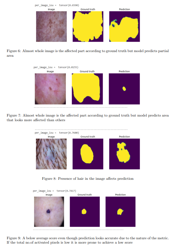
Though the model achieved a high Jaccard Index on the test data, the average score was pulled down due to a few specific scenarios. Some of them are mentioned in figures 6–9.

References

• https://www.kaggle.com/datasets/surajghuwalewala/ham1000-segmentation-and-classification
• Basak, H., Kundu, R., Sarkar, R. (2022). MFSNet: A multi-focus segmentation network for skin lesion segmentation. Pattern Recognition, 128, 108673. https://doi.org/10.1016/j.patcog.2022.108673
• https://www.labellerr.com/blog/semantic-vs-instance-vs-panoptic-which-image-segmentation-technique-to-choose/
• Pham, H. N., Koay, C. Y., Chakraborty, T., Gupta, S., Tan, B. L., Wu, H., Vardhan, A., Nguyen, Q. H., Palaparthi, N. R., Nguyen, B. P., H. Chua, M. C. (2019). Lesion Segmentation and Automated Melanoma Detection using Deep Convolutional Neural Networks and XGBoost. 2019 International Conference on System Science and Engineering (ICSSE). https://doi.org/10.1109/icsse.2019.8823129

 

Join thousands of data leaders on the AI newsletter. Join over 80,000 subscribers and keep up to date with the latest developments in AI. From research to projects and ideas. If you are building an AI startup, an AI-related product, or a service, we invite you to consider becoming a sponsor.

Published via Towards AI