Homography Matrix
Last Updated on July 25, 2023 by Editorial Team
Author(s): Erika Lacson
Originally published on Towards AI.
Introduction to Image Processing with Python
Episode 8: Homography Matrix

Welcome back! U+1F64C We’re near the end of our series, but I still have more to share. This time, we are turning the spotlight on one of my favorite topics in image processing — Homography Matrix! U+1F4AAU+1F5BC️
Fasten your seatbelts because this is going to be a thrilling ride! U+1F680 Let’s jump right in!
Our journey begins with a deep dive into the homography matrix. As a fundamental tool in image processing, it plays a crucial role in capturing geometric transformations in an image. More specifically, it’s the mathematician’s secret weapon for understanding and manipulating perspective transformations. U+1F9D0
Whether you’re interested in aligning images, creating panoramas, or just want to understand the intrinsic geometry of a scene, the homography matrix is a concept you’ll find incredibly useful.
Homography is defined as the mapping between two planar projections of an image. It is represented by a 3×3 transformation matrix in a homogenous coordinates space. These transformations can be a combination of rotation, translation, scaling, or skew operations.
To illustrate:

The documentation for the transform in skimage summarizes these transforms neatly in this link.
However, these examples explicitly defines the transform. What if we are given the input and output image? Depending on the transform, we would need several points to compute for our homography matrix. Let’s do it!
As usual, let’s import the necessary libraries and set the scene for our Homography Matrix exploration:
# Import libraries
from skimage.io import imread, imshow
import matplotlib.pyplot as plt
import numpy as np
from skimage import transform
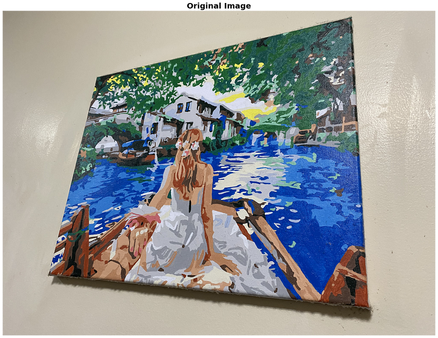
# Display the original image

image = imread('painting.png')
plt.figure(figsize=(20,20))
plt.imshow(image)
plt.title('Original Image', fontsize=20, weight='bold')
plt.axis('off')
plt.show()

Now we want to have a top down view of this painting. We would need to compute for the homography matrix. We have to determine the corners of the painting. In this case, I used paint app to identify the coordinates:
# Source points
src = np.array([879, 625, # top left
 431, 2466, # bottom left
 3251, 61, # top right
 3416, 2767]).reshape((4, 2)) # bottom right
To perform a homography transformation, we’ll need a set of destination points that correspond to the source points. These destination points represent where we want the source points to be in the output image. For a top-down view, we might want the minimum and maximum x and y values of the source points:
# Destination points
dst = np.array([
 [np.min(src[:, 0]), np.min(src[:, 1])], # top left
 [np.min(src[:, 0]), np.max(src[:, 1])], # bottom left
 [np.max(src[:, 0]), np.min(src[:, 1])], # top right
 [np.max(src[:, 0]), np.max(src[:, 1])], # bottom right
])
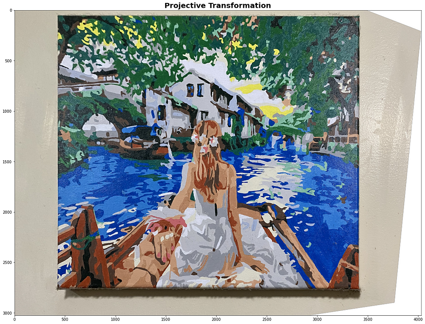
We know that the transformation is projective, so we use that as our parameter:
tform = transform.estimate_transform('projective', src, dst)
tf_img = transform.warp(image, tform.inverse)
fig, ax = plt.subplots(figsize=(20,20))
ax.imshow(tf_img)
_ = ax.set_title('projective transformation')

Considering that the output looks weird with added white pixels outside the wall, we can edit out code to crop the wall and the extra pixels altogether:
# Load the image
image = imread('painting.png')

# Source points
src = np.array([879, 625, # top left
 431, 2466, # bottom left
 3251, 61, # top right
 3416, 2767]).reshape((4, 2)) # bottom right

# Estimate the width and height from the source points
width = np.max(src[:, 0]) - np.min(src[:, 0])
height = np.max(src[:, 1]) - np.min(src[:, 1])

# Destination points (forming a box shape)
dst = np.array([
 [0, 0],
 [0, height],
 [width, 0],
 [width, height]
])

# Compute the projective transform
tform = transform.estimate_transform('projective', src, dst)

# Apply the transformation
warped_image = transform.warp(image, tform.inverse, output_shape=(height, width))

# Convert the warped image to uint8
warped_image_uint8 = (warped_image * 255).astype(np.uint8)

# Display the transformed and cropped image
plt.figure(figsize=(20,20))
plt.imshow(warped_image_uint8)
plt.title('Transformed and Cropped Image', fontsize=20, weight='bold')
plt.axis('off')
plt.show()

There you have it, a pretty and clean looking top-down view of a painting.
Once we have the homography matrix, we can also use it to transform one image to align with the perspective of another image. This can be useful for applications like image stitching (think panorama photos U+1F3DE️), or aligning images for comparison or subtraction. The possibilities are endless!
Conclusion
In this episode, we’ve taken a deep dive into the world of Homography Matrices, a powerful tool in the realm of image transformations.
Stay tuned for our last episode, where we continue this exciting journey through the cosmos of image processing! Until then, keep exploring, keep learning, and remember — in the world of image processing, the only limit is your imagination! U+1F680
References:
- Borja, B. (2023). Lecture 8: Homography Matrix and Texture Metrics [Jupyter Notebook]. Introduction to Image Processing 2023, Asian Institute of Management.
Join thousands of data leaders on the AI newsletter. Join over 80,000 subscribers and keep up to date with the latest developments in AI. From research to projects and ideas. If you are building an AI startup, an AI-related product, or a service, we invite you to consider becoming a sponsor.
Published via Towards AI
Towards AI Academy
We Build Enterprise-Grade AI. We'll Teach You to Master It Too.
15 engineers. 100,000+ students. Towards AI Academy teaches what actually survives production.
Start free — no commitment:
→ 6-Day Agentic AI Engineering Email Guide — one practical lesson per day
→ Agents Architecture Cheatsheet — 3 years of architecture decisions in 6 pages
Our courses:
→ AI Engineering Certification — 90+ lessons from project selection to deployed product. The most comprehensive practical LLM course out there.
→ Agent Engineering Course — Hands on with production agent architectures, memory, routing, and eval frameworks — built from real enterprise engagements.
→ AI for Work — Understand, evaluate, and apply AI for complex work tasks.
Note: Article content contains the views of the contributing authors and not Towards AI.


