


Graph Neural Networks for Fraud Detection in Crypto Transactions
Last Updated on January 6, 2023 by Editorial Team
Last Updated on September 1, 2022 by Editorial Team
Author(s): Maria Zorkaltseva
Originally published on Towards AI the World’s Leading AI and Technology News and Media Company. If you are building an AI-related product or service, we invite you to consider becoming an AI sponsor. At Towards AI, we help scale AI and technology startups. Let us help you unleash your technology to the masses.
In this tutorial, we will apply Graph Convolutional Network (GCN) and Graph Attention Network (GAT) to detect fraudulent bitcoin transactions. Also, we will compare their performances.
Table of Contents
- Introduction
- Spectral-based Convolutional GNN
- Attention-based spatial Convolutional GNN
- Dataset
- Node classification with GCN/GAT using PyTorch Geometric (PyG)
- References
Introduction
Despite significant progress within deep learning areas such as computer vision, natural language/audio processing, time series forecasting, etc., the majority of problems work with non-euclidian geometric data and as an example of such data are social network connections, IoT sensors topology, molecules, gene expression data and so on. The non-Euclidian nature of data implies that all properties of Euclidian vector space R^n can not be applied to such data samples; for example, shift-invariance, which is an important property for Convolutional Neural Networks (CNN), does not save her. In [1] the authors explain how convolution operation can be translated to the non-Euclidian domain using spectral convolution representation for graph structures. At present, Graph Neural Networks (GNN) have found their application in many areas:
- physics (particle systems simulation, robotics, object trajectory prediction)
- chemistry and biology (drug and protein interaction, protein interface prediction, cancer subtype detection, molecular fingerprints, chemical reaction prediction)
- combinatorial optimizations (used to solve NP-hard problems such as traveling salesman problem, minimum spanning trees)
- traffic networks (traffic prediction, taxi demand problem)
- recommendation systems (links prediction between users and content items, social network recommendations)
- computer vision (scene graph generation, point clouds classification, action recognition, semantic segmentation, few-shot image classification, visual reasoning)
- natural language processing (text classification, sequence labeling, neural machine translation, relation extraction, question answering)
Among the classes of state-of-the-art GNNs, we can distinguish them into recurrent GNNs, convolutional GNNs, graph autoencoders, generative GNNs, and spatial-temporal GNNs.
In this tutorial, we will consider the semi-supervised node classification problems using Graph Convolutional Network and Graph Attention Network and compare their performances on the Elliptic dataset, which contains crypto transaction data. Also, we will highlight their building block concepts, which come from spectral-based and spatial-based representations of convolution.
Spectral-based Convolutional GNN
Spectral-based models take their mathematical basis from the graph signal processing field; among known models are ChebNet, GCN, AGCN, and DGCN. To understand the principle of such models, let’s consider the concept of spectral convolution [2, 3].
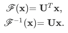
Let’s say we have a graph signal x from R^n, which is the feature vector of all nodes of a graph, and x_i is a value of a i-th node. This graph signal is first transformed to the spectral domain by applying Fourier transform to conduct a convolution operator. After the convolution, the resulting signal is transformed back using the inverse graph Fourier transform. These transforms are defined as:
Here U is the matrix of eigenvectors of the normalized graph Laplacian
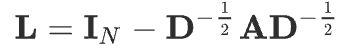
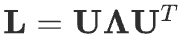
where D is the degree matrix, A is the adjacency matrix of the graph, and I_N is the identity matrix. The normalized graph Laplacian can be factorized as
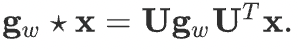
Based on the convolution theorem, the convolution operation with filter g can be defined as:
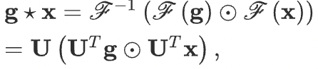
if we denote a filter as g as a learnable diagonal matrix of U^T*g, then we get
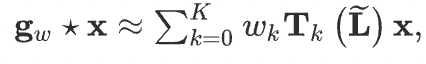
We can understand g_w as a function of the eigenvalues of L. Evaluation of multiplication with the eigenvector matrix U takes O(N²) time complexity; to overcome this problem, in ChebNet and GCN, Chebyshev polynomials are used. For ChebNet, spectral convolution operation is represented as follows.
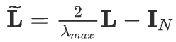
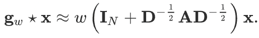
To circumvent the problem of overfitting, in GCN, Chebyshev approximation with K=1 and lambda_max = 2 is used. And convolutional operator will become as follows.

Assuming, w = w_0 = -w_1, we get
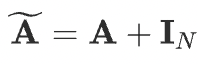
GCN further introduces a normalization trick to solve the exploding/vanishing gradient problem
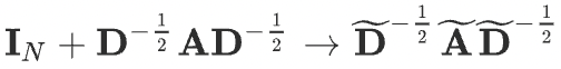

Finally, the compact form of GCN is defined as
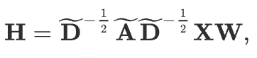
Here X is the input feature matrix, dim(X) = N x F^0, N is the number of nodes, and F^0 number of input features for each node;
A is the adjacency matrix, dim(A) = N x N;
W is the weights matrix, dim(W) = F x F’, F is the number of input features, F’ is the number of output features;
H represents a hidden layer of graph neural network, dim(H) = N x F’.
At each i-th layer H_i, features are aggregated to form the next layer’s features, using the propagation rule f (e.g. sigmoid/relu), and thus features become increasingly abstract at each consecutive layer, which reminds the principle of CNN.
Attention-based spatial Convolutional GNN
Among spatial-based convolutional GNN models, the following models are widely known: GraphSage, GAT, MoNet, GAAN, DiffPool, and others. The working principle is similar to CNN convolution operator application to image data, except the spatial approach applies convolution to differently sized node neighbors of a graph.
Attention mechanism gained wide popularity thanks to the models used in NLP tasks (e.g., LSTM with attention, transformers). In the case of GNN having an attention mechanism, contributions of neighboring nodes to the considered node are neither identical nor pre-defined, as, for example, in GraphSage or GCN models.
Let’s look at the attention mechanism of GAT [4]; normalized attention coefficients for this model can be calculated via the following formula:
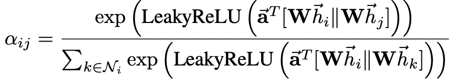
Here, T represents transposition and || is concatenation operation;
h is a set of node features (N is a number of nodes, F is a number of features in each node)

W is weight matrix (linear transformation to a features), dim(W) = F’ x F
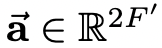
Vector a is the weight vector for a single-layer feed-forward neural network
The softmax function ensures that the attention weights sum up to one overall neighbour of the i-th node.
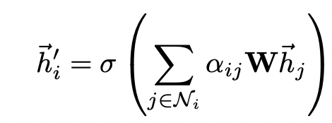
Finally, these normalized attention coefficients are used to compute a linear combination of the features corresponding to them, to serve as the final output features for every node.
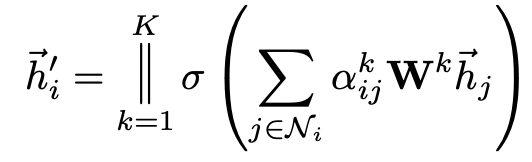
Usage of single self-attention can lead to instabilities, and in this case, multi-head attention with K independent attention mechanisms is used
Dataset
Here, for the node classification task, we will use the Elliptic dataset. Dataset consists of 203 769 nodes and 234 355 edges. There are three categories of nodes: “licit”, “illicit”, or “unknown”. A node is deemed “licit” / “illicit” if the corresponding transaction has been created by an entity that belongs to a licit (exchanges, wallet providers, miners, financial service providers, etc.) or illicit (scams, malware, terrorist organizations, ransomware, Ponzi schemes, etc.) category respectively. A detailed description of that dataset is available in the following article, “The Elliptic Data Set: opening up machine learning on the blockchain”.
Node classification with GCN/GAT using PyTorch Geometric (PyG)
Here we will consider a semi-supervised node classification problem using PyG library, where nodes will be transactions and edges will be transactions flows.
You can simply import the Elliptic bitcoin dataset from PyG pre-installed datasets using the instructions down below, but for the sake of clarity, let’s build PyG dataset object by ourselves. Raw data can be downloaded via this link.
from torch_geometric.datasets import EllipticBitcoinDataset
dataset = EllipticBitcoinDataset(root=’./data/elliptic-bitcoin-dataset’)
Data loading/preparation
For the data preparation, I used this Kaggle notebook as a basis.
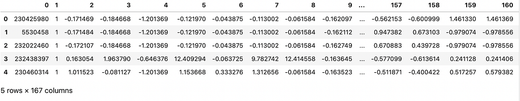
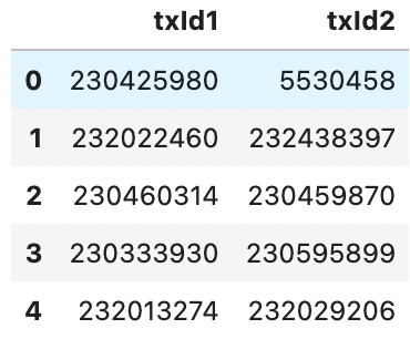
# here column 0 stands for node_id, column 1 is the time axis
df_features.head()
df_edges.head()
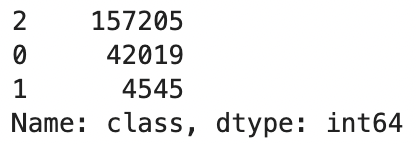
df_classes.head()

0 — legitimate
1 — fraud
2 — unknown class
df_classes['class'].value_counts()
Preparing edges
Total amount of edges in DAG: torch.Size([2, 234355])
Preparing nodes
Let’s ignore the temporal axis and consider the static case of fraud detection.
PyG Dataset
Number of nodes: 203769
Number of node features: 165
Number of edges: 234355
Number of edge features: 165
Average node degree: 1.15
Number of classes: 2
Has isolated nodes: False
Has self loops: False
Is directed: True
Train dataset size: 39579
Validation dataset size: 6985
Test dataset size: 157205
Models
Train/test helpers
Train GCN
Epoch   0 | Train Loss: 0.759 | Train Acc:  62.16% | Val Loss: 0.73 | Val Acc: 64.07%
Saving model for best loss
Epoch  10 | Train Loss: 0.307 | Train Acc:  86.43% | Val Loss: 0.30 | Val Acc: 87.16%
Saving model for best loss
Epoch  20 | Train Loss: 0.258 | Train Acc:  89.52% | Val Loss: 0.25 | Val Acc: 89.61%
Saving model for best loss
Epoch  30 | Train Loss: 0.244 | Train Acc:  90.49% | Val Loss: 0.24 | Val Acc: 90.32%
Saving model for best loss
Epoch  40 | Train Loss: 0.230 | Train Acc:  91.32% | Val Loss: 0.22 | Val Acc: 91.40%
Saving model for best loss
Epoch  50 | Train Loss: 0.219 | Train Acc:  91.85% | Val Loss: 0.22 | Val Acc: 91.77%
Saving model for best loss
Epoch  60 | Train Loss: 0.214 | Train Acc:  92.35% | Val Loss: 0.21 | Val Acc: 92.61%
Saving model for best loss
Epoch  70 | Train Loss: 0.210 | Train Acc:  92.60% | Val Loss: 0.21 | Val Acc: 92.80%
Saving model for best loss
Epoch  80 | Train Loss: 0.201 | Train Acc:  92.86% | Val Loss: 0.20 | Val Acc: 92.81%
Saving model for best loss
Epoch  90 | Train Loss: 0.195 | Train Acc:  93.15% | Val Loss: 0.20 | Val Acc: 92.81%
Saving model for best loss
Epoch 100 | Train Loss: 0.194 | Train Acc:  93.25% | Val Loss: 0.19 | Val Acc: 93.53%
Saving model for best loss
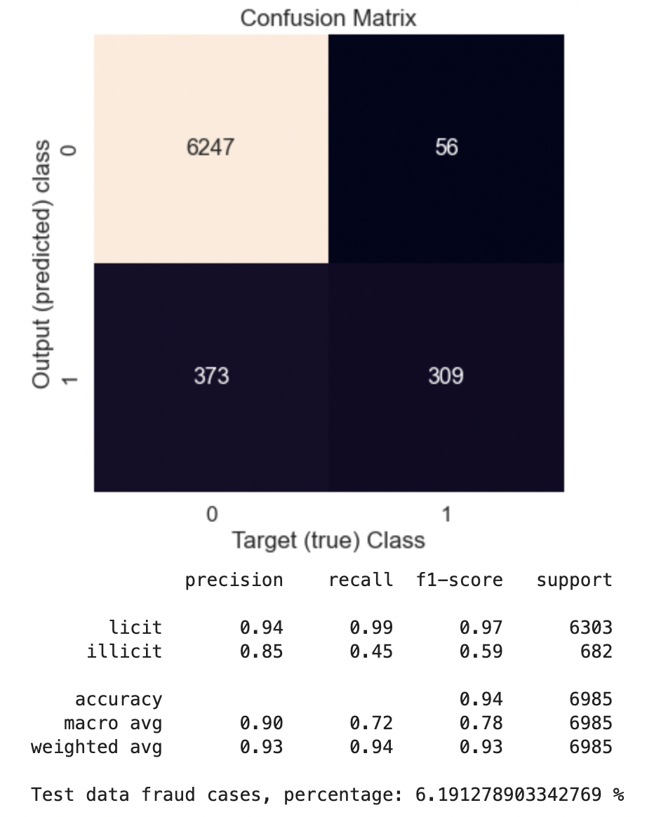
Test GCN
Train GAT
Epoch   0 | Train Loss: 1.176 | Train Acc:  68.34% | Val Loss: 1.01 | Val Acc: 68.33%
Saving model for best loss
Epoch  10 | Train Loss: 0.509 | Train Acc:  88.63% | Val Loss: 0.48 | Val Acc: 88.70%
Saving model for best loss
Epoch  20 | Train Loss: 0.489 | Train Acc:  90.09% | Val Loss: 0.49 | Val Acc: 89.94%
Epoch  30 | Train Loss: 0.465 | Train Acc:  89.87% | Val Loss: 0.48 | Val Acc: 89.76%
Saving model for best loss
Epoch  40 | Train Loss: 0.448 | Train Acc:  89.81% | Val Loss: 0.44 | Val Acc: 90.15%
Saving model for best loss
Epoch  50 | Train Loss: 0.445 | Train Acc:  90.04% | Val Loss: 0.44 | Val Acc: 89.89%
Epoch  60 | Train Loss: 0.443 | Train Acc:  90.22% | Val Loss: 0.44 | Val Acc: 90.45%
Epoch  70 | Train Loss: 0.439 | Train Acc:  90.38% | Val Loss: 0.43 | Val Acc: 90.16%
Saving model for best loss
Epoch  80 | Train Loss: 0.426 | Train Acc:  90.57% | Val Loss: 0.43 | Val Acc: 90.41%
Saving model for best loss
Epoch  90 | Train Loss: 0.423 | Train Acc:  90.72% | Val Loss: 0.42 | Val Acc: 90.38%
Saving model for best loss
Epoch 100 | Train Loss: 0.418 | Train Acc:  90.72% | Val Loss: 0.42 | Val Acc: 90.74%
Saving model for best loss
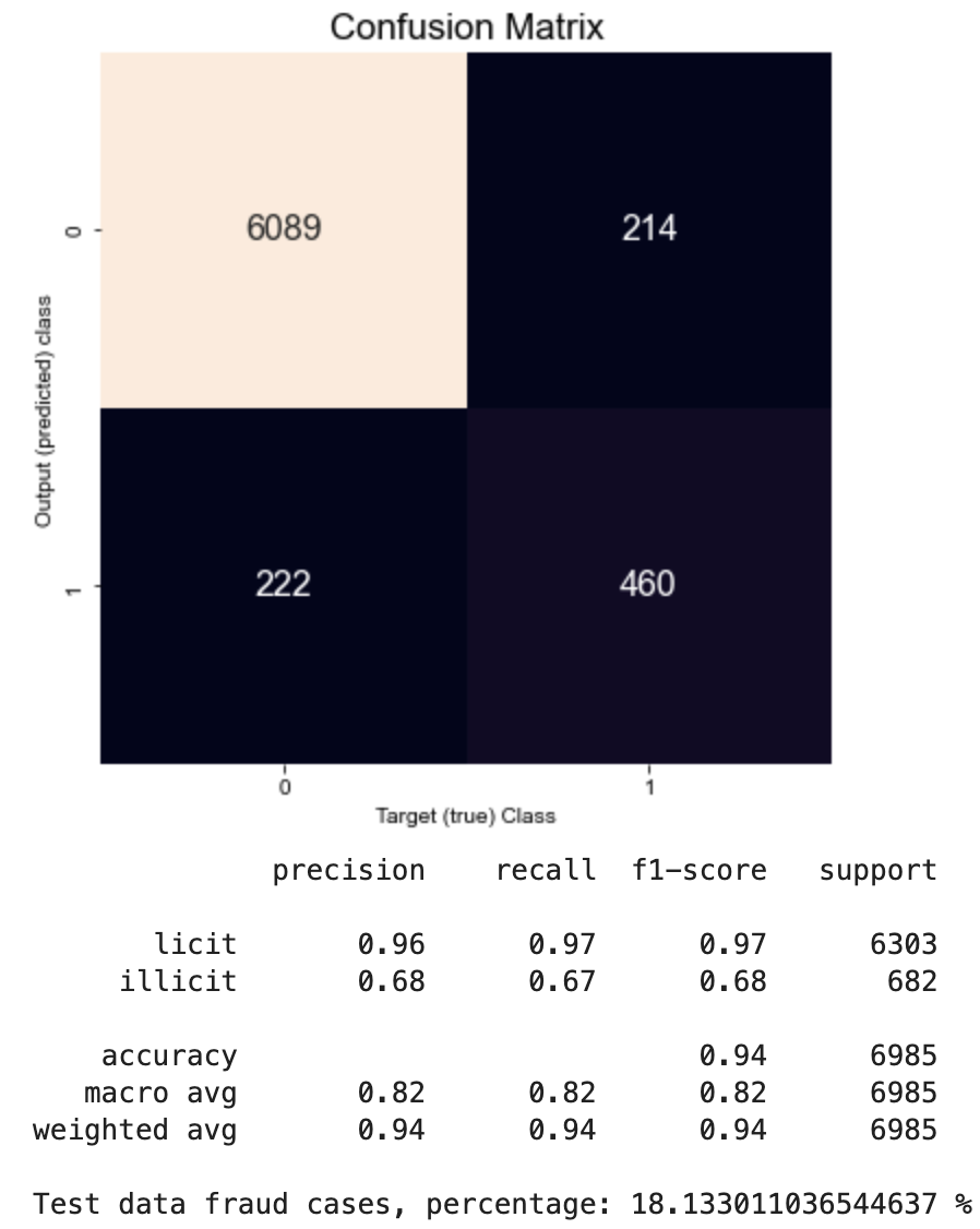
Test GAT
👉🏻 Full code is also accessible through my GitHub.
Conclusion
From the calculation results, we can see that the GAT model converges slower in comparison to GCN, and train/validation accuracies are slightly lower than GCN. However, the confusion matrix built from validation data (labeled data) shows that the recall metric improved from 0.45 (GCN) to 0.67 (GAT). Thus, the GAT model more clearly identifies fraudsters than GCN but is also more strict with licit cases. Tests on unlabelled data containing 157205 samples show that in the case of GCN, there are only 6 % of fraud cases, while in the case of GAT, this amount is about 18 %.
References
References
- Bronstein M. et al., Geometric deep learning: going beyond Euclidean data (2017), IEEE SIG PROC MAG, https://arxiv.org/pdf/1611.08097.pdf
- Kipf T. N., Welling M. Semi-supervised classification with graph convolutional networks (2017), ICLR, https://arxiv.org/pdf/1609.02907.pdf
- Zhou J. et al., Graph neural networks: A review of methods and applications (2020), AI Open, Volume 1, https://doi.org/10.1016/j.aiopen.2021.01.001
- Velickovic P. et al., Graph Attention Networks (2018), ICLR, https://arxiv.org/pdf/1710.10903.pdf
Graph Neural Networks for Fraud Detection in Crypto Transactions was originally published in Towards AI on Medium, where people are continuing the conversation by highlighting and responding to this story.
Join thousands of data leaders on the AI newsletter. It’s free, we don’t spam, and we never share your email address. Keep up to date with the latest work in AI. From research to projects and ideas. If you are building an AI startup, an AI-related product, or a service, we invite you to consider becoming a sponsor.
Published via Towards AI
Towards AI Academy
We Build Enterprise-Grade AI. We'll Teach You to Master It Too.
15 engineers. 100,000+ students. Towards AI Academy teaches what actually survives production.
Start free — no commitment:
→ 6-Day Agentic AI Engineering Email Guide — one practical lesson per day
→ Agents Architecture Cheatsheet — 3 years of architecture decisions in 6 pages
Our courses:
→ AI Engineering Certification — 90+ lessons from project selection to deployed product. The most comprehensive practical LLM course out there.
→ Agent Engineering Course — Hands on with production agent architectures, memory, routing, and eval frameworks — built from real enterprise engagements.
→ AI for Work — Understand, evaluate, and apply AI for complex work tasks.
Note: Article content contains the views of the contributing authors and not Towards AI.
Related posts
Recent Posts


")