


Gradient Descent Optimization
Last Updated on January 6, 2023 by Editorial Team
Last Updated on October 18, 2022 by Editorial Team
Author(s): Rohan Jagtap
Originally published on Towards AI the World’s Leading AI and Technology News and Media Company. If you are building an AI-related product or service, we invite you to consider becoming an AI sponsor. At Towards AI, we help scale AI and technology startups. Let us help you unleash your technology to the masses.
Gradient Descent Optimization Algorithms
Most deep learning algorithms train by optimizing some kind of objective (or loss) function. We typically try to either maximize or minimize these functions. Gradient-based optimization is the most extensively used technique for training neural networks.
In this article, we will see the well-known Gradient Descent algorithm. We will discuss what it is, why it works, and finally, implement a gradient descent optimizer for TensorFlow.
This article is for anyone who has just heard about Gradient Descent or someone who thinks of Gradient Descent as a black box and has a shallow understanding of what happens but wants to delve deeper into why things are the way they are.
Note: This article is inspired by the ‘The Deep Learning textbook: Chapter 4: Numerical Computation’ and the ‘Stanford CS class CS231n: Convolutional Neural Networks for Visual Recognition notes.’
Contents
This a rather very long article, and all of these sections might not interest or concern the audience at once. Please feel free to use the following list to navigate and skip to the parts that are relevant to you:
- The Loss Function
- Optimization
1. Random Search
2. Random Local Search
3. Gradient-based Optimization - Gradient Descent
1. The Minima
2. Why can’t we just equate the derivative to 0 and solve for x?
3. Parameter Update Formula
a. Why is the negative gradient the direction of the steepest descent?
b. Why do we say ‘going in the opposite direction of the gradient?’ - Jacobians and Hessians
1. Second Derivative Test and Second-Order Optimization
2. Why not use second-order optimization algorithms for neural nets? - Computing the Gradient
1. Using finite differences
2. Using Calculus - Implementation
- Conclusion
- References
The Loss Function
A loss function, which also goes by the names objective function, error function, cost function, or criterion, can be any (differentiable) function that helps evaluate an algorithm’s output against the ground truth. It can be anything from the Mean Squared Error for continuous values to Cross-entropy loss for probability distributions. While loss functions are very interesting, today, we are only concerned with how to minimize them.
To understand what we exactly want, let’s visualize a loss function. In practice, many parameters vary the loss making it hard to visualize. For simplicity, we will consider just 2.
Let’s define a loss: y = L(x, z) where x, y, z are Cartesian coordinates along the X, Y, and Z axes, respectively.
Let’s take random values wx and wz for which we get the point in space: (wx, yw, wz).
Now, we can either vary some m randomly as ywₘ = L(wx + m, z) which will give us a line plot for the loss values yw along the xy-plane, or we can vary some m and n as ywₘₙ = L(wx + m, z + n) which will give us a three-dimensional plot. Here’s what it looks like for the Multiclass SVM loss:
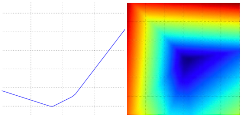
So what we ultimately want is to find some wx* and wz* such that yw (i.e., the loss) is the least (the darkest blue point). Starting from arbitrary values and working our way down to these ‘optimal’ values is called optimization.
Optimization
In the previous section, we saw what exactly optimization in this context is. Now let’s see how we can go about this and understand what gradient-based optimization is and why it is used to train neural networks.
First, let’s think about some easy ways to do this:
Random Search
Let’s pick values randomly and keep track of values that give the best loss:
x*, z* = 0, 0
bestloss = inf
for a few iterations
    x, z = random(), random()
    y = L(x, z)
    if y < bestloss then
        bestloss, x*, z* = y, x, z
There are infinitely many points in the coordinate space, and the odds of ending up with the optimal values are very low. So this is a pretty bad approach. Let’s see if we can do better.
Random Local Search
We can do something similar to what we did while visualizing the loss function. We can start with random values, generate some small random Δx, Δz, and add them to x and z respectively. If the new values improve the loss, we keep them:
x*, z* = random(), random()
bestloss = inf
for a few iterations
    Δx, Δz = random(), random()
    x, z = x* + Δx, z* + Δz
    y = L(x, z)
    if y < bestloss then
        bestloss, x*, z* = y, x, z
Analogy: Think of this as a blindfolded hiker trying to climb down a hill, probing every step before advancing.
While it looks good, this approach is still very random and lacks structure. Moreover, an even bigger issue is it’s very expensive. In the worst case, one might have to probe every point on the function, which might not even be possible.
Gradient-based Optimization
Let’s go back to high school and recall elementary calculus. For a function y = f(x), the derivative f'(x) or dy/dx is defined as the rate of change of y w.r.t. small changes in x. It is also the slope of f(x) at point x.
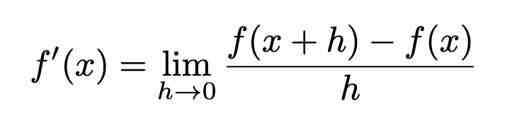
The interpretation and explanation of this expression is out of the scope of today’s discussion, but if you watch closely, you will find that it is pretty self-explanatory. It can also be seen as the standard slope formula.
We can further solve for f(x + h) and approximate it to:
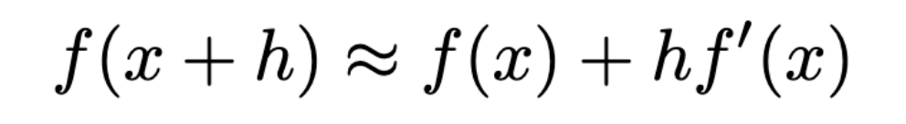
Many textbooks and papers assume the above expression. So this is where it comes from.
From the above expression, we can solve and conclude that:
for a small enough ϵ, f(x — ϵ sign(f’(x))) is smaller than f(x)
So it looks like by using derivatives like the above, we can take a ‘small enough’ ϵ and reduce f(x) in small steps by updating x. This technique is called Gradient Descent.
This example, however, was a univariate function. Typically, we will deal with multivariate functions (sometimes with millions of variables in the case of neural nets). Each variable represents the magnitude of the function in a given ‘direction.’ So for multivariate functions, we take partial derivatives, i.e., individual derivatives w.r.t. each direction (or variable).
The gradient, ∇ f is nothing but a vector of all the partial derivatives of a function
We will discuss Gradient Descent in greater detail in the next section.
Gradient Descent
So far, we’ve seen how we can minimize a function. Now let’s think about where to stop, i.e., how do we know if we have arrived at the ‘minimum’ value of the function?
The Minima
f’(x) = 0 defines the points where the slope is 0. In two dimensions, these are the points where the slope of a function is parallel to the x-axis and thus is 0. Similar ideas follow in higher dimensions. These points are called critical or stationary points. Since the derivative is 0, there is no information about which direction to move.
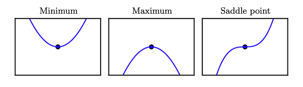
- A point that gives the absolute lowest value of f(x) is a global minimum. Whereas a local minimum is a point where f(x) is lower than all the neighboring points.
Since the derivative here is 0, we cannot make a move towards much lower values of f(x). - Vice versa is true for the global and local maximum.
- Finally, a saddle point is neither a minimum nor a maximum.
It is worthwhile to note that the Multiclass SVM loss function we saw earlier belongs to a type of function called the Convex function. There is a separate subfield of mathematical optimization dedicated to convex optimization.
On the contrary, a neural network is highly non-linear, and the losses are highly non-convex. It means that the concepts we derive for convex functions may not be as easily applicable in the case of neural networks.
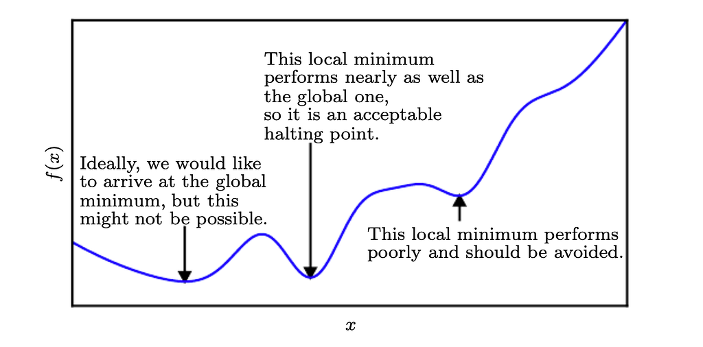
For instance, a strictly convex function has no more than one minimum. However, in the context of deep learning, we are dealing with very complex loss functions that might have multiple local and global minimums and most likely are bumpy terrains— making gradient descent non-trivial.
Therefore, it is very difficult or, in some cases, even impossible to reach a global minimum. So we settle for a very low value of loss which might not even be a minimum:
So when f'(x) = 0, if we are at the extremities of the function, one might have a very valid question:
Why can’t we just equate the derivative to 0 and solve for x?
Isn’t this what we were taught in high school? So what’s wrong with it? Is iterative gradient descent really necessary?
Well, no! We can indeed live without it.
But let’s consider this — in the case of classic linear regression, equating the derivative of the cost function to zero and solving for the parameters involves inverting a matrix (Here’s why). Even the most efficient techniques for this have a complexity of O(n³), where n is the number of parameters.
Now with neural networks, we are talking about millions of parameters. Moreover, it is a much more complex function than linear regression. So it will be even more difficult to solve. To add to it, these losses may or may not be differentiable everywhere.
Iterative methods like Gradient Descent offer a much more practical and reasonably efficient solution to these problems.
Of course, if it’s any easier or faster, we can always equate the derivative to 0.
Parameter Update Formula
Till now, we’ve discussed what we exactly want, then we talked about various approaches to go about and fixated on one, then we saw what the stopping condition looks like. Now let’s see how to actually solve for x at every step.
To start with, let’s first take a step back and recall what we deduced about f(x — ϵ sign(f’(x))). This value will be less than f(x) given ϵ is small enough. Let’s take a moment and think about x — ϵ sign(f’(x)) — if f’(x) is positive, then our new x will be x — ϵ, and if f’(x) is negative, then x will be x + ϵ. So we are basically just using the derivative for its sign and reversing it.
In most textbooks/papers/articles on gradient descent, when they say ‘going in the opposite direction of the gradient,’ this is what they mean.
However, this is just one variable. In practice, we are dealing with millions of them. So does this apply in the multivariate case? If yes, how? Let’s find out.
Note that from now on, we will represent x as a collective set of multiple parameters (variables). So,
x = (x₁, x₂, x₃, …, xₙ) and
f(x) = f(x₁, x₂, x₃, …, xₙ)
Since we are dealing with vectors, we will need directional derivatives.
The components of the gradient vector ∇ₓf(x) represent the rates of change of the function f(x) w.r.t each of its variables xᵢ. However, we wish to know how f(x) changes as its variables change along any direction from a given point.
So the directional derivative of a function f(x) in a direction υ (a unit vector), at a point x, is given by the partial derivative of f(x + αυ) w.r.t α., i.e., ∂f(x + αυ)/∂α when α = 0. Basically, the rate of change of f(x + αυ) with small changes in α because υ is just a direction vector and cannot change. Let’s solve this:
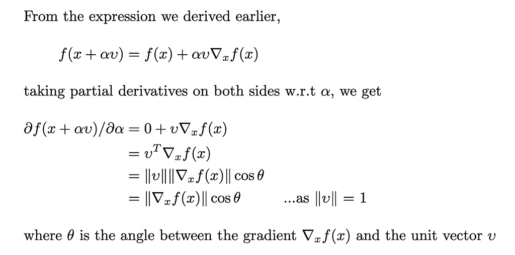
From the above, we can say that for any given direction υ, the directional derivative is proportional to the cosine of the angle between the gradient of the function f(x) at point x and the direction itself.
Now in the context of gradient descent, we can take a unit vector in any possible direction at a given point x and move in that direction. However, it is desirable to move in a direction where the f decreases the fastest. For this, the directional derivative must be the highest but in the reverse direction, i.e., the rate of change of the function with small changes in x should be greatest in the direction of -υ. This will happen when the cosθ value is -1. So we have to pick a υ for which the θ = π. This is nothing but the vector -∇ₓf(x).
Using this and the earlier idea, we can come up with the following update:
x' = x - ϵ ∇ₓf(x) ... where ϵ is the learning rate
Generally, we pick a very small value for ϵ. Sometimes we can solve for ϵ such that υᵀ∇ₓf(x') = 0. Think of this as walking down a hill until you reach a point where you start walking upwards again (Since υᵀ∇ₓf(x') = 0, cosθ = 0, and hence, υ and ∇ₓf(x') are orthogonal). Another strategy is to evaluate x’ for a few arbitrary values of ϵ and pick the one which gives the smallest value for f(x'). This strategy is called line search.
This is known as the method of steepest descent or gradient descent.
Jacobians and Hessians
So far, we’ve used the gradient ∇ₓf(x) for multivariate functions that take vectors as input (x = (x₁, x₂, …, xₙ)), and output scalars (y = f(x)). However, while dealing with functions that input as well as output vectors,
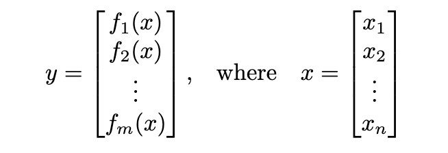
we use a Jacobian matrix. It is a matrix of all the partial derivatives:
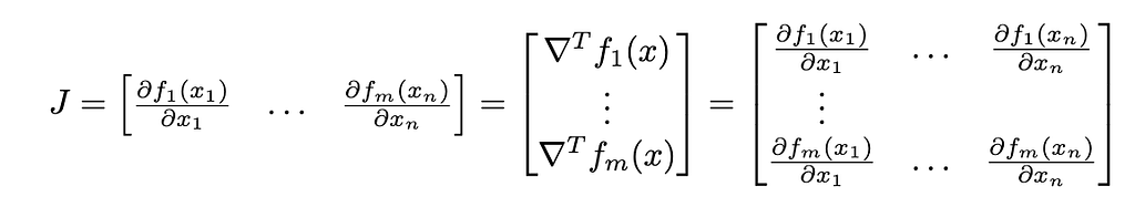
This is particularly useful while applying the Chain Rule.
Now, if we take a derivative of a derivative, we get a second derivative or a second-order derivative (f”(x)). This quantity will tell us how the first-order derivative changes as we vary the input. We can think of the second
derivative as measuring curvature.
The use of second-order derivatives is beyond the scope of this article, so we will briefly see what it is:
Second Derivative Test and Second-Order Optimization
If the function is a line, just the gradient is sufficient to tell about its curvature (i.e., if slope < 0 then the function descends; if slope > 0 then it ascends; and slope = 0 means a flat line, as discussed earlier). Otherwise, we can use the second derivative. For example, for a quadratic function, the derivative is a line, so we can take the derivative of the derivative and use the above analogy.
This is particularly useful for evaluating critical points f’(x) = 0. Here, if the second derivative f”(x) > 0, then as we move towards the right, f’(x) it increases and decreases as we go to the left. This means we are at the local minimum. Similarly, when f”(x) < 0, we are at the local maximum. However, unfortunately, when f”(x) = 0, it is inconclusive if it is a saddle point or a flat surface. However, in multiple dimensions, it is actually possible to find positive evidence of saddle points in some cases. This is known as the second derivative test.
In the case of multiple dimensions or multivariate functions, we have the Hessian matrix. These are like Jacobians but with second derivatives. Also, it is true that a Hessian is a Jacobian of the gradient.
Now, if you notice, with the information about the curvature of the function, we can actually determine a correct step size for our parameter update, which won’t overshoot our function value. We can do this by including the Hessian matrix in the optimization. One of the simplest methods that do this is called Newton’s Method:
x' = x - H⁻¹∇f
This belongs to a whole family of algorithms that use the Hessian matrix — second-order optimization algorithms. On the other hand, the ones that use the gradient are called first-order optimization algorithms.
Why not use second-order optimization algorithms for neural nets?
They are very expensive in terms of speed and memory. For constructing the hessian matrix, we need the derivative of all the combinations of variables and gradients, which is O(n²).
Moreover, it is very difficult to implement second derivatives and much more complex. Here is a list of other issues with second-order optimization algorithms, which makes them infeasible to apply to neural networks.
Computing the Gradient
We can do this in two ways: the finite differences formula and using calculus.
Using finite differences
We can directly apply the formula we saw earlier for all partial derivatives. However, it is recommended to use a modified version instead:
f'(x) = (f(x + h) − f(x − h)) / 2h
This one explores both sides of the point x. To calculate the gradient:
enumerate all parameters with i
    backup = x[i]

    x[i] = backup - h
    fxminush = f(x)

    x[i] = backup + h
    fxplush = f(x)

    x[i] = backup

    gradient[i] = (fxplush - fxminush) / 2h
The obvious downside of this method is that it is approximate. Moreover, the above loop will run for every single update. So basically, if we have a million parameters and one thousand steps, this will run for 1000 * 1000000 iterations. This is very expensive and is used only for gradient check sanity tests.
Using Calculus
Instead of using the approximate formula, we can apply the direct formula for the derivative of the function. After that, we can obtain the gradient using this derivative, which can be directly used in the update step.
However, this is not how exactly modern machine learning libraries work — instead, they use automatic differentiation. The idea is that all the operations we do are ultimately a sequence or a combination of elementary arithmetic (addition, subtraction, multiplication, division) operations and elementary functions (sin, cos, log, etc.). So one can record the sequence of execution and apply the Chain Rule.
Implementation
Finally, let’s try to implement an optimizer for TensorFlow. For more on implementing custom optimizers in TensorFlow, see this.
To test this, I trained a model for a simple MNIST classification against the built-in SGD optimizer first and then this one and compared the results:
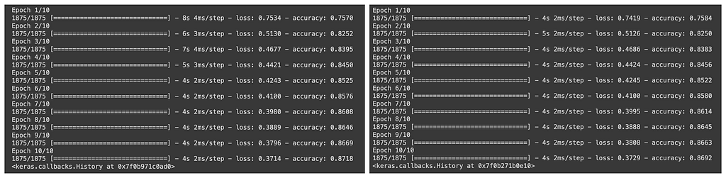
We can see that it works fine.
Conclusion
In this rather exhaustive article,
- We discussed the need for optimization. Then, we saw a few optimization strategies and introduced gradient-based optimization algorithms.
- We talked about the gradient descent algorithm and answered a few why’s and what’s w.r.t gradient descent. We also derived the expression for parameter update.
- We then briefly touched on Jacobians, Hessians, and the idea of second-order optimization algorithms.
- We saw how to calculate the gradient for any given function and compared a few approaches.
- And finally, we implemented a simple gradient descent optimizer for TensorFlow.
References
- Deep Learning
- CS231n Convolutional Neural Networks for Visual Recognition
- Why is gradient descent required?
Why the gradient is the direction of steepest ascent: https://www.khanacademy.org/math/multivariable-calculus/multivariable-derivatives/gradient-and-directional-derivatives/v/why-the-gradient-is-the-direction-of-steepest-ascent
- Why second order SGD convergence methods are unpopular for deep learning?
- Basic classification: Classify images of clothing | TensorFlow Core
- tf.keras.optimizers.Optimizer | TensorFlow v2.10.0
Gradient Descent Optimization was originally published in Towards AI on Medium, where people are continuing the conversation by highlighting and responding to this story.
Join thousands of data leaders on the AI newsletter. It’s free, we don’t spam, and we never share your email address. Keep up to date with the latest work in AI. From research to projects and ideas. If you are building an AI startup, an AI-related product, or a service, we invite you to consider becoming a sponsor.
Published via Towards AI
Towards AI Academy
We Build Enterprise-Grade AI. We'll Teach You to Master It Too.
15 engineers. 100,000+ students. Towards AI Academy teaches what actually survives production.
Start free — no commitment:
→ 6-Day Agentic AI Engineering Email Guide — one practical lesson per day
→ Agents Architecture Cheatsheet — 3 years of architecture decisions in 6 pages
Our courses:
→ AI Engineering Certification — 90+ lessons from project selection to deployed product. The most comprehensive practical LLM course out there.
→ Agent Engineering Course — Hands on with production agent architectures, memory, routing, and eval frameworks — built from real enterprise engagements.
→ AI for Work — Understand, evaluate, and apply AI for complex work tasks.
Note: Article content contains the views of the contributing authors and not Towards AI.
Related posts
Recent Posts
")


")


