Getting a Grip on Data and Model Drift with Azure Machine Learning

Author(s): Andreas Kopp

Originally published on Towards AI the World’s Leading AI and Technology News and Media Company. If you are building an AI-related product or service, we invite you to consider becoming an AI sponsor. At Towards AI, we help scale AI and technology startups. Let us help you unleash your technology to the masses.

Getting a Grip on Data and Model Drift With Azure Machine Learning

By Natasha Savic and Andreas Kopp

Change is the only constant in life. In machine learning, it shows up as drift of data, model predictions, and decaying performance, if not managed carefully.

In this article, we discuss data and model drift and how it affects the performance of production models. You will learn methods to identify and to mitigate drift and MLOps best practices to transition from static models to evergreen AI services using Azure Machine Learning.

We also include a sample notebook if you want to try out the concepts in practical examples.

Understanding data and model drift

Many machine learning projects conclude after a phase of extensive data and feature engineering, modeling, training, and evaluation with a satisfactory model that is deployed to production. However, the longer a model is in operation, the more problems can creep in that might remain undetected for quite a long time.

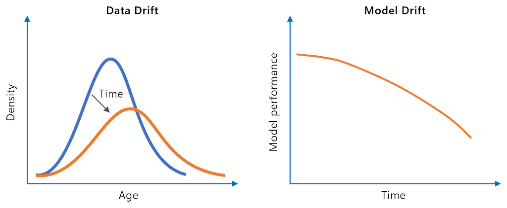
Data drift means that distributions of input data change over time. Drift can lead to a gap between what the model has initially learned from the training data and the inferencing observations during production. Let’s look at a few examples of data drift:

• Real-world changes: an originally small demographic group increasingly appears in the labor market (e.g., war refugees); new regulatory frameworks come into play influencing user consent (e.g., GDPR)
• Data acquisition problems: incorrect measurements due to a broken IoT sensor; an initially mandatory input field of a web form becomes optional for privacy reasons
• Data engineering problems: unintended coding or scaling changes or swap of variables

Model drift is accompanied by a decrease in model performance over time (e.g., accuracy drop in a supervised classification use case). There are two main sources of model drift:

• Real-world changes are also referred to as concept drift: The relationship between features and target variables has changed in the real world. Examples: the collapse of travel activities during a pandemic and; rise of inflation impacts buying behavior.
• Data drift: The described drift of input data might also affect model quality. However, not every occurrence of data drift is necessarily a problem. When drift occurs on less important features the model might respond robustly, and performance is not affected. Let us assume that a demographic cohort (a specific combination of age, gender, and income) occurs more often during inferencing than seen during training. It won’t cause headaches if the model still predicts the outcomes for this cohort correctly. It is more problematic if the drift leads the model into less populated and/or more error-prone areas of the feature space.

Model drift typically stays undetected until new ground truth labels are available. The original test data is no longer a reliable benchmark because the real-world function has changed.

The following illustration summarizes the various kinds of drift:

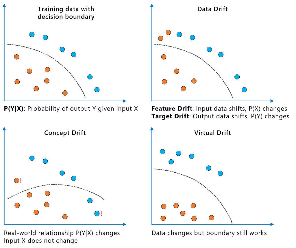
The transition from normal behavior to drift can be vastly different. Demographic changes in the real world typically lead to gradual data or model drift. However, a broken sensor might cause abrupt deviations from the normal range. Seasonal fluctuations in buying behavior (e.g., Christmas season) are manifested as a recurring drift.

If we have timestamps for our observations (or the data points are at least arranged chronologically), the following can be done to detect, analyze and mitigate drift.

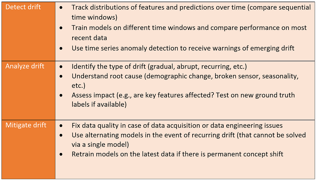
We will describe these methods in more detail below and experiment with them using a predictive maintenance case study.

From static to evergreen models

The options to analyze and mitigate data and model drift depend on the availability of current data over the machine learning model’s lifecycle.

Let us assume that a bank collected historical data to train a model to support credit lending decisions. The goal is to predict whether a loan application should be approved or rejected. Labeled training data was collected in the period from January to December 2020.

The bank’s data scientists have spent the first quarter of 2021 training and evaluating the model and decided to bring it to production in April 2021. Let us look at three options the team can use for collecting production data:

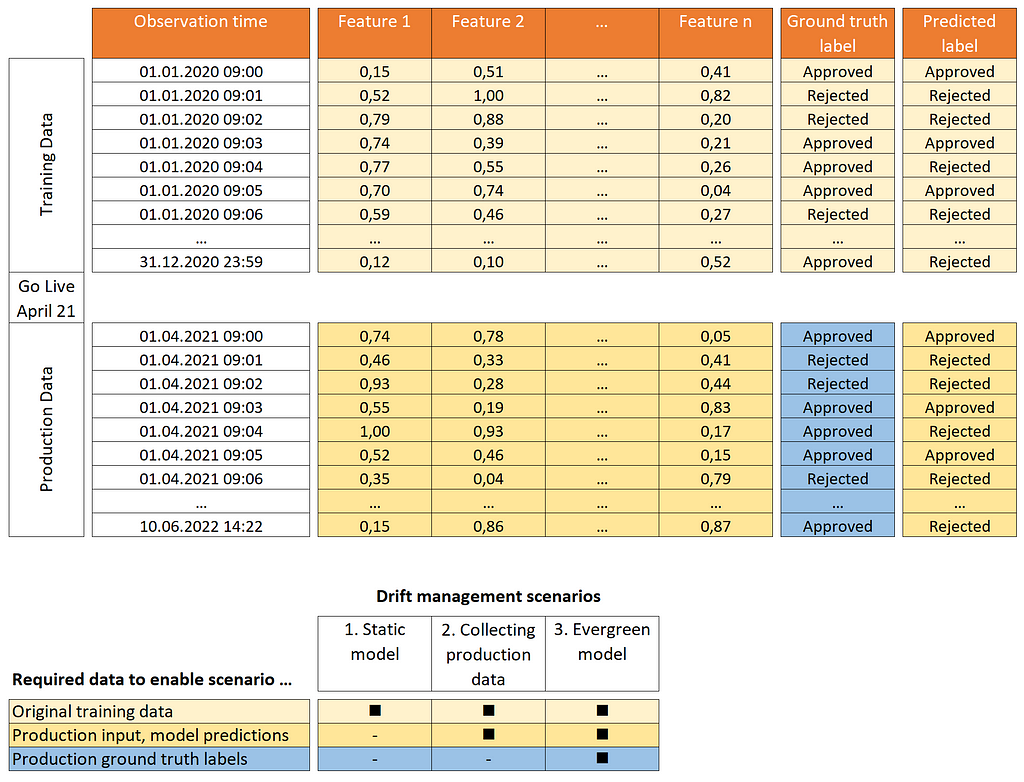
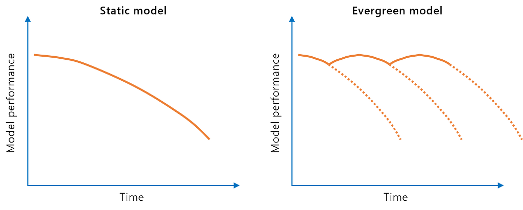
Scenario 1: Static model

Here, the team doesn’t collect any production data. Perhaps they did not consider this at all since their project scope only covered delivering the initial model. Another reason could be open data privacy questions (storing regulated personal data).

Obviously, there is not much that can be done to detect data or model drift beyond analyzing the historical training data. Drift may only be uncovered when model users start complaining about the model predictions are becoming increasingly unsuitable for business decisions. However, since feedback is not systematically collected, gradual drift will likely remain undiscovered for a long time.

Interestingly, many productive machine learning models are run in this mode today. However, machine learning lifecycle management procedures like MLOps are getting more traction in practice to address issues like these.

The static model approach might be acceptable if the model is trained on representative data and the feature/target relationship is stable over time (e.g., biological phenomena which change at an evolutionary pace).

Scenario 2: Collecting production data

The team decides to collect observed input data (features) from the production phase together with the corresponding model predictions.

This approach is straightforward to implement if there are no data protection concerns or other organizational hurdles. By comparing the recent production data with original training observations, drift in features and predicted labels can be found. Significant shifts in key features (in terms of feature importance) can be used as a trigger for further investigation.

However, essential information is missing to find out if there is a problem with the model: we do not have new ground truth labels to evaluate the production predictions. This might lead to the following situations:

• Virtual drift (false positive): We observe data drift, but the model still works as desired. This may get the team to acquire new labeled data for retraining although it is unnecessary (from a model drift perspective).
• Concept drift (false negative): While there is no drift in the input data, the real-world function has moved away from what the model had learned. Hence, an increasingly outdated model leads to inaccurate business decisions.

Scenario 3: Evergreen model

In this scenario, the bank not only analyzes production input and predictions for potential drift but also collects labeled data. Depending on the business context, this can be done in one of the following ways:

• Business units contribute newly labeled data points (as was done for the initial training)
• Human-in-the-loop feedback: The model predictions from the production phase are systematically reviewed. Especially false approvals and false rejections, found by domain experts, and the corresponding features with the corrected labels are collected for retraining.

Incorporating human-in-the-loop feedback requires adjustment of processes and systems (e.g., business users can overwrite or flag incorrect predictions in their applications).

The main advantages are that concept drift can be identified with high reliability and the model can regularly be refreshed by retraining.

Incorporating business feedback and regular retraining is an essential part of mature MLOps practices (see our reference architecture example for Azure Machine Learning below).

Data and model drift management in practice

It is essential to have a detection mechanism that measures drift systematically. Ideally, such a mechanism is part of an integrated MLOps workflow that compares training and inference distributions on a continuous basis. We have compiled several mechanisms that support data and model drift management.

We are using a predictive maintenance use case based on a synthetic dataset in our sample notebook. The goal is to predict equipment failure based on features like speed or heat deviations, operator, assembly line, days since the last service, etc.

To identify drift, we combine statistical techniques and distribution overlaps (data drift) as well as predictive techniques (model/concept drift). For both drift types, we will briefly introduce the method used.

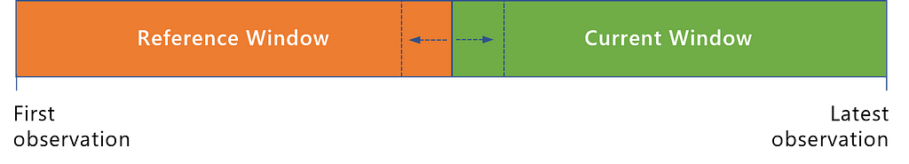
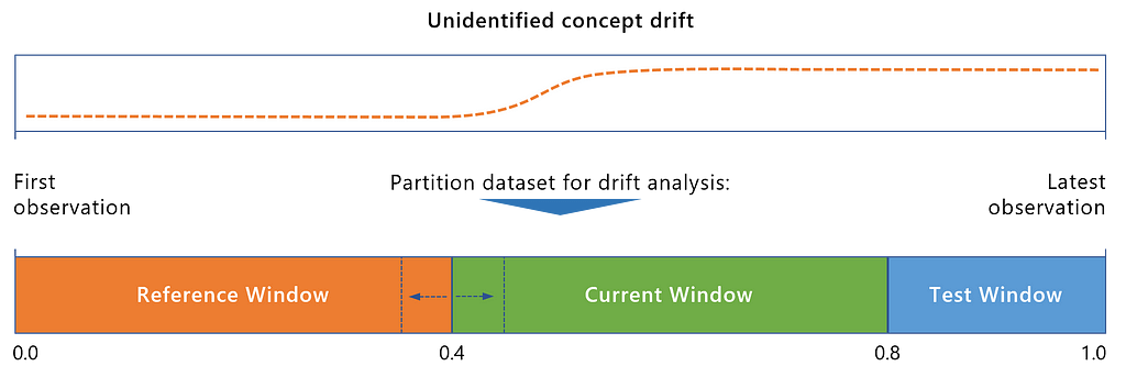
Drift detection starts by partitioning a dataset of chronologically sorted observations into a reference and current window. The reference (or baseline) window represents older observations and is often identical to the initial training data. The current window typically reflects more recent data points seen in the production phase. This is not a strict 1:1 mapping as it might be needed to adjust the windows to better locate when drift occurred.

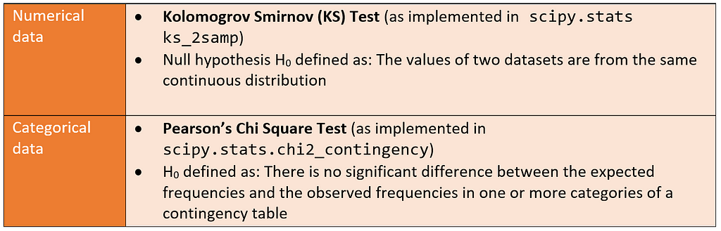
We first need to differentiate between numerical and categorical/discrete data. For the statistical tests, both types of data will undergo distinct non-parametric tests that provide a p-value. We are handling different sample sizes and do not make assumptions about the actual distribution of our data. Therefore, non-parametric approaches are a handy way to test the similarity of two samples without needing to know the actual probability distribution.

Those tests allow us to accept or reject the null hypothesis with a degree of confidence, as defined by the p-value. As such, you can control the sensitivity of the test by adjusting the threshold for the p-value. We recommend a more conservative p-value such as 0.01 by default. The larger your sample gets, the more prone it is to pick up on noise. Other commonly used methods to figure out the drift between distributions are the Wasserstein Distance for continuous and the JS Divergence for probability distributions.

Here are some best practices to limit the number of false alarms in drift detection:

1. Scope the drift analyses to a shortlist of key features if you have many variables in your dataset
2. Use a sub-sample instead of all data points if your dataset is large
3. Reduce the p-value threshold further or select an alternative test for larger data volumes

While statistical tests are useful to identify drift, it is hard to interpret the magnitude of the drift as well as in which direction it occurs. Given a variable like age, did the sample get older or younger and how is the age spread? To answer those questions, it is useful to visualize the distributions. For this, we add another non-parametric method: the Kernel Density Estimation (KDE). Since we have two different data types, we will perform a pre-processing step on the categorical data to convert it into a pseudo-numerical notation by encoding the variables. The same ordinal encoder object is used for both the reference and the current distributions to ensure consistency:

Now that we have encoded our data, we can visually inspect either the entire dataset or selected variables of interest. We use the Kernel Density Estimation functions of the reference and current samples to compute their intersection in percent. The following steps were adapted from this sample:

1. Pass the data into a KDE function as in scipy.stats.gaussian_kde() with the bandwidth method “scott”. The parameter determines the degree of smoothing of the distribution.
2. Take the range (min and max of both distributions) and compute the intersection points of both KDE functions within this range by using the differential of both functions.
3. Perform pre-processing for variables that have a constant value to avoid errors and align the scale of both distributions.
4. Approximate the area under the intersection points using the composite trapezoidal rule as per numpy.trapz().
5. Plot the reference and current distributions, intersection points as well as the area of intersection with the percentage of overlap.
6. Add the respective statistical test (KS or Chi-Square) to the title and provide a drift indication (Drift vs. No Drift)

The steps can be understood in more depth by checking out the code samples. The result of the KDE intersections looks as follows:

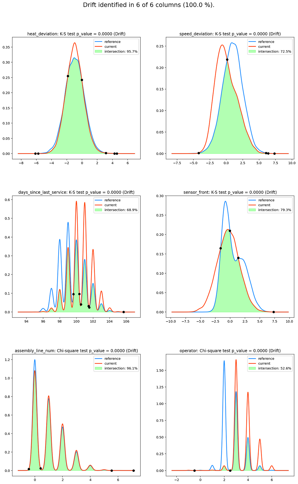
A brief inspection of the plots tells us:

1. Which variables have significantly different distributions between the reference and current sample?
2. What is the magnitude and direction of the drift?

If we look at the variable “operator”, we can see that there was a substantial change in terms of which employee was operating the machine between when the model was fitted versus today. For example, it could have happened that an operator has retired and, consequently, does not operate any machines anymore (operator 2). Conversely, we see that new operators have joined who were not present before (e.g., operator 6).

Now that we have seen how to uncover drift in features and labels, let us find out if the model is affected by data or concept drift.

Similar to before, we stack the historical (training) observations and recently labeled data points together in a chronological dataset. Then, we compare model performance based on the most recent observations, as the following overview illustrates.

At the core, we want to answer the question: Does a newer model perform better in predicting on most recent data than a model trained on older observations?

We probably have no idea in advance if and where drift has crept in.

Therefore, in our first attempt, we might use the original training data as reference and the inference observations as current windows. If we find the existence of drift by this, we will likely try out different reference and current windows to pinpoint where exactly drift crept in.

A couple of options exist for predictive model drift detection:

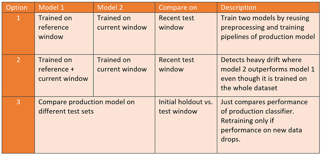
Each option has specific advantages. As a result of the first alternative, you already have a trained candidate ready for deployment if model 2 outperforms model 1. The second option will likely reduce false positives, at the expense of being less sensitive to drift. Alternative 3 reduces unnecessary training cycles in cases where no drift is identified.

Let’s check out how to use option 1 to find drift in our predictive maintenance use case. The aggregated dataset consists of 45,000 timestamped observations which we spilt into 20,000 references, 20,000 current, and 5,000 most recent observations for the test.

We define a scikit-learn pipeline to preprocess numerical and categorical features and train two LightGBM classifiers for comparison:

After repeating the last step for the current classifier, we compare the performance metrics to find out if there is a noticeable gap between the models:

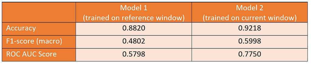
The current model outperforms the reference model by a large margin. Therefore, we can conclude that we indeed have identified model drift and that the current model is a promising candidate for replacing the production model. A visual way of inspection is to compare the distributions of confidence scores of both classifiers:

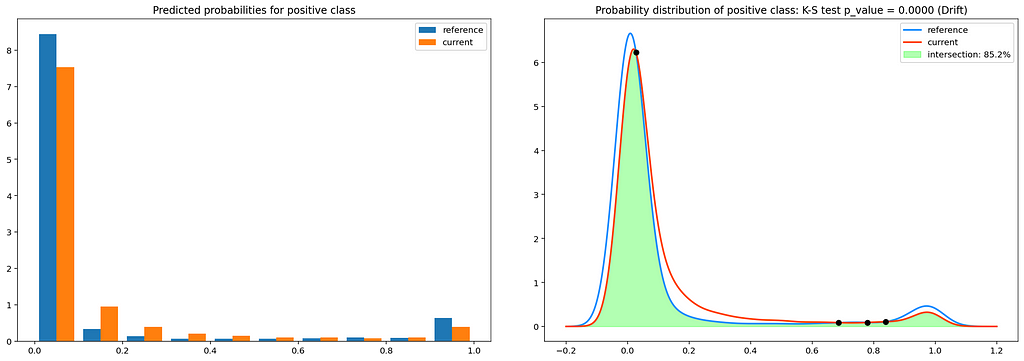
The histograms on the left show a clear difference between the predicted class probabilities of the reference and current models and therefore also confirm the existence of model drift.

Finally, we reuse our KDE plots and statistical tests from the data drift section to measure the extent of the drift. The intersection between the KDE plots for both classifiers amounts to only 85%. Furthermore, the results of the KS test suggest that the distributions are not identical.

In this example, the results were to be expected because we intentionally built drift into our synthetic predictive maintenance dataset. With a real-world dataset, results won’t always be as obvious. Also, it might be necessary to try different reference and current window splits to reliably find model drift.

MLOps reference architecture for evergreen models

We will now focus on embedding drift detection and mitigation in an MLOps architecture with Azure Machine Learning. The following section leverages concepts such as Azure ML Datasets, Models, and Pipelines. The demo repository provides an example of an Azure ML pipeline for generating the data drift detection plots. To automate the re-training of models, we recommend using the latest Azure MLOPs code samples and documentation. The following illustration provides a sample architecture including everything we learned about data and model drift so far.

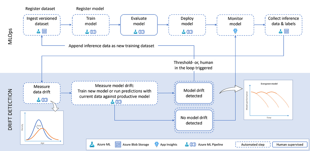
By considering drift mitigation as part of an automated Azure MLOps workflow, we can maintain evergreen ML services with manageable effort. To do so, we perform the following steps:

1. Ingest and version data in Azure Machine Learning
   This step is crucial to maintain a lineage between the training data, machine learning experiments, and the resulting models. For automation, we use Azure Machine Learning pipelines which consume managed datasets. By specifying the version parameter (version=”latest”) you can ensure to obtain the most recent data.
2. Train model
   In this step, the model is trained on the source data. This activity can also be part of an automated Azure Machine Learning pipeline. We recommend adding a few parameters like the dataset name and version to re-use the same pipeline object across multiple dataset versions. By doing so, the same pipeline can be triggered in case model drift is present. Once the training is finished, the model is registered in the Azure Machine Learning model registry.
3. Evaluate model
   Model evaluation is part of the training/re-training pipeline. Besides looking at performance metrics to see how good a model is, a thorough evaluation also includes reviewing explanations, checking for bias and fairness issues, looking at where the model makes mistakes, etc. It will often include human verification.
4. Deploy model
   This is where you deploy a specific version of the model. In the case of evergreen models, we would deploy the model that was fitted to the latest dataset.
5. Monitor model
   Collection of telemetry about the deployed model. For example, an Azure AppInsights workbook can be used to collect the number of requests made to the model instance as well as service availability and other user-defined metrics.
6. Collect inference data and labels
   As part of a continuous improvement of the service, all the inferences that are made by the model should be saved into a repository (e.g., Azure Data Lake) alongside the ground truth (if available). This is a crucial step as it allows us to figure out the amount of drift between the inference and the reference data. Should the ground truth labels not be available, we can monitor data drift but not model drift.
7. Measure data drift
   Based on the previous step, we can kick off the data drift detection by using the reference data and contrasting it against the current data using the methods introduced in the sections above.
8. Measure model drift
   In this step, we determine if the model is affected by data or concept drift. This is done using one of the methods introduced above.
9. Trigger re-training
   In case of model or concept drift, we can trigger a full re-training and deployment pipeline utilizing the same Azure ML pipeline we used for the initial training. This is the last step that closes the loop between a static and an evergreen model. The re-training triggers can either be:
   Automatic — Comparing performance between the reference model and current model and automatically deploying if the current model performance is better than the reference model.
   Human in the loop — Inspect data drift visualization alongside performance metrics between reference and current model and deploy with a data scientist/ model owner in the loop. This scenario would be suitable for highly regulated industries. This can be done using PowerApps, Azure DevOps pipelines, or GitHub Actions.

Next steps

In this article, we have looked at practical concepts to find and mitigate the drift of data and machine learning models for tabular use cases. We have seen these concepts in action using our demo notebook with the predictive maintenance example. We encourage you to adapt these methods to your own use cases and appreciate any feedback.

Being able to systematically identify and manage the drift of production models is a big step toward mature MLOps practices. Therefore, we recommend integrating these concepts into an end-to-end production solution like the MLOps reference architecture introduced above. The last part of our notebook includes examples of how to implement drift detection using automated Azure Machine Learning Pipelines.

Data and model drift management is only one building block of a holistic MLOps vision and architecture. Feel free to check out the documentation for general information about MLOps and how to implement it using Azure Machine Learning.

In our examples, we have looked at tabular machine learning use cases. Drift mitigation approaches for unstructured data like images and natural language are also emerging. The Drift Detection in Medical Imaging AI repository provides a promising method of analyzing medical images in conjunction with metadata to detect model drift.

---

Getting a Grip on Data and Model Drift with Azure Machine Learning was originally published in Towards AI on Medium, where people are continuing the conversation by highlighting and responding to this story.

Join thousands of data leaders on the AI newsletter. It’s free, we don’t spam, and we never share your email address. Keep up to date with the latest work in AI. From research to projects and ideas. If you are building an AI startup, an AI-related product, or a service, we invite you to consider becoming a sponsor.

Published via Towards AI