Geometric Transformations on Images

Author(s): Akula Hemanth Kumar

Originally published on Towards AI.

Making computer vision easy with Monk, low code Deep Learning tool and a unified wrapper for Computer Vision

Table of contents

1. Scaling
2. Translation
3. Rotation
4. Affine Transformation
5. Perspective Transformation

Scaling

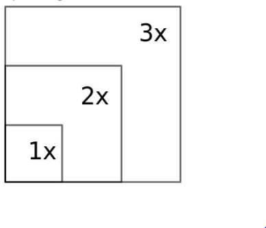
• Image scaling refers to the resizing of a digital image.
• The magnification of digital material is known as upscaling.
• The downsizing is known as downscaling.

• Ideal Scenario- Lossless transformation.
• Image resolution- height(in pixels) , *width(in pixels)

Image resizing using numpy

import numpy as np
import cv2
from matplotlib import pyplot as plt
img = cv2.imread("imgs/chapter4/tessellate.jpg", -1)
print("Input image shape - {}".format(img.shape))
plt.imshow(img[:,:,::-1])
plt.show()

Output

Input image shape - (240, 320, 3)

Downscaling width

height, width, channels = img.shape

# create blank image of half the width
resized_img_width = np.zeros((height, width//2, channels), dtype=np.int32)for r in range(height):
 for c in range(width//2):
 resized_img_width[r][c] += (img[r][2*c])
 
print("Width resized image shape - {}".format(resized_img_width.shape))
plt.imshow(resized_img_width[:,:,::-1])
plt.show()

Output

Width resized image shape - (240, 160, 3)

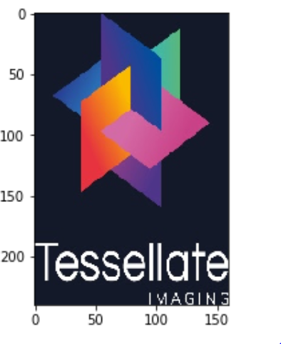
Downscaling image to half its width and height

resized_img = np.zeros((height//2, width//2, channels), dtype=np.int32)for r in range(height//2):
 for c in range(width//2):
 resized_img[r][c] += (resized_img_width[r*2][c])
print("Complete resized image shape - {}".format(resized_img.shape))
plt.imshow(resized_img[:,:,::-1])
plt.show()

Output

Complete resized image shape - (120, 160, 3)

Upscaling height

half_upsclaled_img = np.zeros((height, width//2, channels), dtype=np.int32)half_upsclaled_img[0:height:2, :, :] = resized_img[:, :, :]
half_upsclaled_img[1:height:2, :, :] = resized_img[:, :, :]
print("Height upscaled image shape - {}".format(half_upsclaled_img.shape))
plt.imshow(half_upsclaled_img[:,:,::-1])
plt.show()

Output

Height upscaled image shape - (240, 160, 3)

Upscaling width

upsclaled_img = np.zeros((height, width, channels), dtype=np.int32)# Expand rows by replicating every consecutive row
upsclaled_img[:, 0:width:2, :] = half_upsclaled_img[:, :, :]
upsclaled_img[:, 1:width:2, :] = half_upsclaled_img[:, :, :]
print("Fully upscaled image shape - {}".format(upsclaled_img.shape))
upscaled_img_manual = upsclaled_img
plt.imshow(upsclaled_img[:,:,::-1])
plt.show()

Output

Fully upscaled image shape - (240, 320, 3)

Comparing original and upscaled

f = plt.figure(figsize=(15,15))
f.add_subplot(1, 2, 1).set_title('Original Image')
plt.imshow(img[:, :, ::-1])
f.add_subplot(1, 2, 2).set_title('Upscaled image post downscaling')
plt.imshow(upsclaled_img[:, :, ::-1])
plt.show()

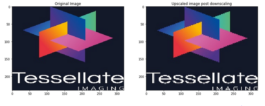
Note: There is a lot of information loss in this sort of image resizing.

Image resizing using OpenCV

• Downscaling shape by using cv2.resize().
• Upscaling shape by using cv2.resize().

Downscaling image to half its width and height

import numpy as np
import cv2
from matplotlib import pyplot as plt
img = cv2.imread("imgs/chapter4/tessellate.jpg", -1)height, width, channels = img.shape

# create blank image of half the width
resized_img = cv2.resize(img, (width//2, height//2))
print("Downscaled image shape - {}".format(resized_img.shape))
plt.imshow(resized_img[:,:,::-1])
plt.show()

Upscaling image to its original width and height

height, width, channels = img.shape

# create blank image of half the widthupscaled_img = cv2.resize(resized_img, (width, height));
print("Upscaled image shape - {}".format(upscaled_img.shape))
upscaled_img_opencv = upscaled_img
plt.imshow(upscaled_img[:,:,::-1])
plt.show()

Output

Upscaled image shape - (240, 320, 3)

Comparing original, manually upscaled, rescaled using opencv

f = plt.figure(figsize=(15,15))
f.add_subplot(3, 1, 1).set_title('Original Image');
plt.imshow(img[:, :, ::-1])
f.add_subplot(3, 1, 2).set_title('Manually Upscaled post downscaling');
plt.imshow(upscaled_img_manual[:, :, ::-1])
f.add_subplot(3, 1, 3).set_title('Upscaled using opencv post downscaling');
plt.imshow(upscaled_img[:, :, ::-1])
plt.show()

Image resizing using Pillow

Downscaling image to half its width and height

import numpy as np
from PIL import Image
from matplotlib import pyplot as plt
img_p = Image.open("imgs/chapter4/tessellate.jpg")width, height = img_p.size

# create blank image of half the width
resized_img = img_p.resize((width//2, height//2))
print("Downscaled image shape - {}".format(resized_img.size))
plt.imshow(resized_img);
plt.show()

Output

Downscaled image shape - (160, 120)

Upscaling image to its original width and height

width, height = img_p.size

# create blank image of half the width
upscaled_img = resized_img.resize((width, height))
print("Upscaled image shape - {}".format(upscaled_img.size))
plt.imshow(resized_img)
plt.show()

Output

Upscaled image shape - (320, 240)

Comparing original, manually upscaled, rescaled using opencv

f = plt.figure(figsize=(15,15))
f.add_subplot(2, 2, 1).set_title('Original Image')
plt.imshow(img[:, :, ::-1])
f.add_subplot(2, 2, 2).set_title('Manually Upscaled post downscaling')
plt.imshow(upscaled_img_manual[:, :, ::-1])
f.add_subplot(2, 2, 3).set_title('Upscaled using opencv post downscaling')
plt.imshow(upscaled_img_opencv[:, :, ::-1])
f.add_subplot(2, 2, 4).set_title('Upscaled using PIL post downscaling')
plt.imshow(upscaled_img)
plt.show()

Algorithms for scaling

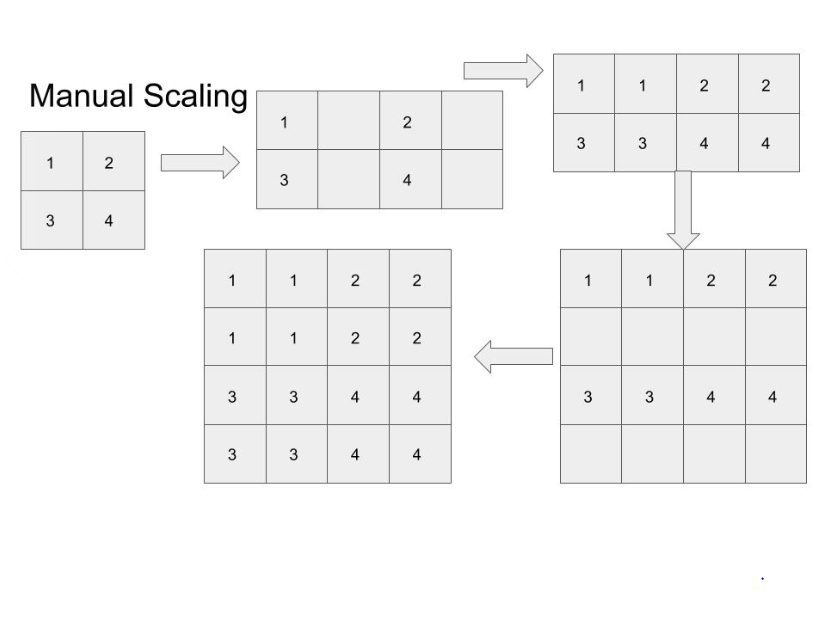
What is Interpolation

• Interpolation is a method of constructing new data points within the range of a discrete set of known data points.
• It is often required to interpolate, i.e estimate the value of that function for an intermediate value of the independent variable.
• It is also called as curve fitting. Approximating values

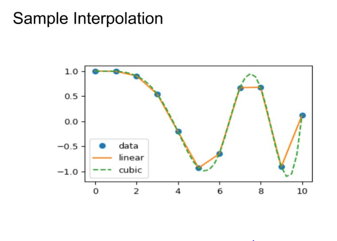
OpenCV Interpolations

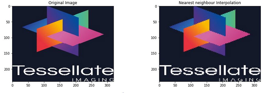
nearest neighbor interpolation

• Assign the value nearest to the current pixel.
• The nearest neighbor is the most basic.
• It requires the least processing time of all the interpolation algorithms because it only considers one pixel- the closest one to the interpolated point.

Bilinear Interpolation

• Bilinear interpolation considers the closest 2*2 neighborhood of known pixel values surrounding the unknown pixel.
• It then takes a weighted average of these 4 pixels to arrive at its final interpolated value.

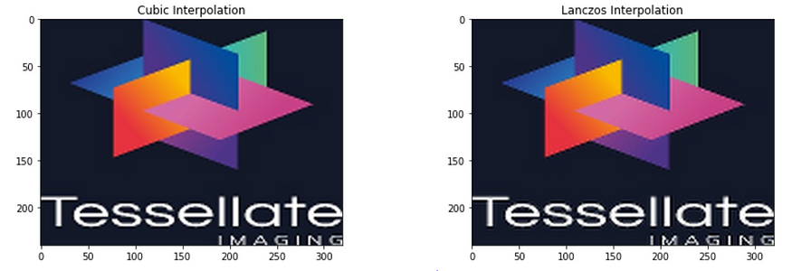
BiCubic Interpolation

LancZos Interpolation

• Higher-order interpolation.
• Works in frequency domain thus hard to visualize.
• A higher dimension filtering and feature extraction methodology.

Which interpolation to use?

• cv2.INTER_LINEAR is used by default.
• cv2.INTER_AREA for shrinking.
• cv2.INTER_CUBIC again for shrinking, better but slow.
• cv.INTER_LINEAR for zooming.
• Other complex ones when the speed of computation is not considered.

OpenCV algorithms

Pillow algorithms

Translation

• Shifting image by certain pixels in either of the four directions.

Why is it required?

• For data Augmentation.

Image translation using basic Numpy

import numpy as np 
import cv2 
from matplotlib import pyplot as plt 
img = cv2.imread("imgs/chapter4/dog.jpg",-1)
plt.imshow(img[:,:,::-1])
plt.show()

Translating to right by 50 pixels

h, w, c = img.shape;
img_new = np.zeros((h, w, c), dtype=np.uint8);

f = plt.figure(figsize=(15,15))
f.add_subplot(3, 1, 1).set_title('Original Image');
plt.imshow(img[:, :, ::-1])
f.add_subplot(3, 1, 2).set_title('New Blank Image');
plt.imshow(img_new[:, :, ::-1])
plt.show()

img_new[:, 50:, :] = img[:, :w-50, :]

plt.imshow(img_new[:,:,::-1])
plt.show()

Translating to left by 50 pixels

h, w, c = img.shape
img_new = np.zeros((h, w, c), dtype=np.uint8)

img_new[:, :w-50, :] = img[:, 50:, :]
plt.imshow(img_new[:,:,::-1])
plt.show()

Translating down by 50 pixels

h, w, c = img.shape
img_new = np.zeros((h, w, c), dtype=np.uint8)

img_new[50:, :, :] = img[:h-50, :, :]
plt.imshow(img_new[:,:,::-1])
plt.show()

Translating up by 50 pixels

h, w, c = img.shape;
img_new = np.zeros((h, w, c), dtype=np.uint8)

img_new[:h-50, :, :] = img[50:, :, :]
plt.imshow(img_new[:,:,::-1])
plt.show()

Rotation

Image rotation using PIL

import numpy as np
from PIL import Image
from matplotlib import pyplot as plt
img_p = Image.open("imgs/chapter4/triangle.jpg")
plt.imshow(img_p)
plt.show()

Clockwise rotation by 30 degrees with pivot as the center

img_p_new = img_p.rotate(-30)
plt.imshow(img_p_new)
plt.show()

Anti-Clockwise rotation by 30 degrees with pivot as the center

img_p_new = img_p.rotate(30)
plt.imshow(img_p_new)
plt.show()

Affine Transformation

• Transformation involving translation and rotations of images.
• But the transformation is done in a way that straight lines in the image are never curved.

Affine Transformation using OpenCV

import numpy as np
import cv2
from matplotlib import pyplot as plt
img = cv2.imread("imgs/chapter4/tessellate.jpg", -1)
plt.imshow(img[:,:,::-1])
plt.show()

Keeping two points static and changing

img = cv2.imread("imgs/chapter4/tessellate.jpg", -1)
rows,cols,ch = img.shape


# Read as x, y
pts1 = np.float32([[50,50],[200,50], [50,200]])
pts2 = np.float32([[80,50],[200,50], [50,200]])


cv2.circle(img,(int(pts1[0][0]),int(pts1[0][1])),5,(0,255,0),-1)
cv2.circle(img,(int(pts1[1][0]),int(pts1[1][1])),5,(0,0,255),-1)
cv2.circle(img,(int(pts1[2][0]),int(pts1[2][1])),5,(255,0,0), -1)M = cv2.getAffineTransform(pts1,pts2)
dst = cv2.warpAffine(img,M,(cols,rows))

f = plt.figure(figsize=(15,15))
f.add_subplot(1, 2, 1).set_title('Input')
plt.imshow(img[:, :, ::-1])
f.add_subplot(1, 2, 2).set_title('Transformed')
plt.imshow(dst[:, :, ::-1])
plt.show()

Keeping 1 point as hinge

img = cv2.imread("imgs/chapter4/tessellate.jpg", -1)
rows,cols,ch = img.shape

pts1 = np.float32([[50,50],[200,50], [50,200]])
#pts2 = np.float32([[60,50],[190,50], [50,200]]) 
# Works as translation + shrinking
pts2 = np.float32([[60,50],[200,50], [50,175]])


cv2.circle(img,(int(pts1[0][0]), int(pts1[0][1])), 5, (0,255,0), -1)
cv2.circle(img,(int(pts1[1][0]), int(pts1[1][1])), 5, (0,0,255), -1)
cv2.circle(img,(int(pts1[2][0]), int(pts1[2][1])), 5, (255,0,0), -1)

M = cv2.getAffineTransform(pts1,pts2)

dst = cv2.warpAffine(img,M,(cols,rows))

f = plt.figure(figsize=(15,15))
f.add_subplot(1, 2, 1).set_title('Input')
plt.imshow(img[:, :, ::-1])
f.add_subplot(1, 2, 2).set_title('Transformed')
plt.imshow(dst[:, :, ::-1])
plt.show()

Translating all three points -> translation

img = cv2.imread("imgs/chapter4/tessellate.jpg", -1)
rows,cols,ch = img.shape

pts1 = np.float32([[50,50],[200,50], [50,200]])
pts2 = np.float32([[60,50],[210,50], [60,200]])


cv2.circle(img,(int(pts1[0][0]), int(pts1[0][1])), 5, (0,255,0), -1)
cv2.circle(img,(int(pts1[1][0]), int(pts1[1][1])), 5, (0,0,255), -1)
cv2.circle(img,(int(pts1[2][0]), int(pts1[2][1])), 5, (255,0,0), -1)

M = cv2.getAffineTransform(pts1,pts2)

dst = cv2.warpAffine(img,M,(cols,rows))

f = plt.figure(figsize=(15,15))
f.add_subplot(1, 2, 1).set_title('Input')
plt.imshow(img[:, :, ::-1])
f.add_subplot(1, 2, 2).set_title('Transformed')
plt.imshow(dst[:, :, ::-1])
plt.show()

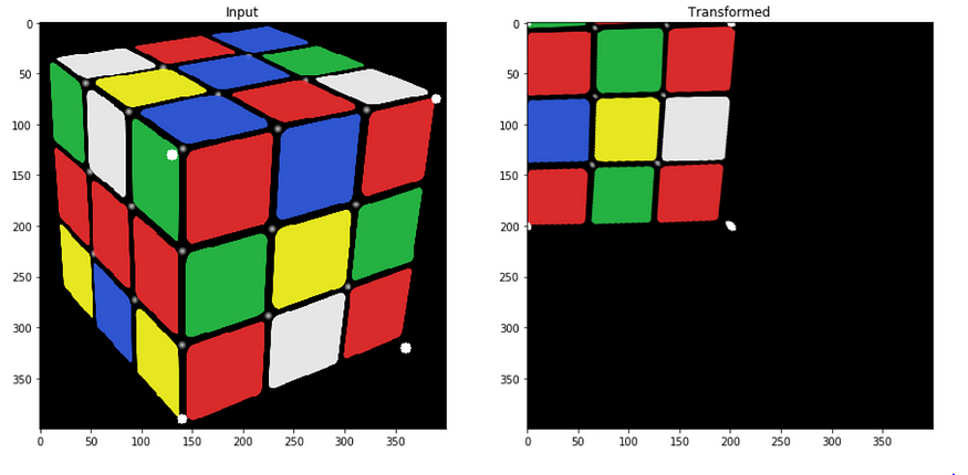
Perspective Transformation

Perspective transform using OpenCV

import numpy as np
import cv2
from matplotlib import pyplot as plt
img = cv2.imread("imgs/chapter4/cube.png", 1)
plt.imshow(img[:,:,::-1])
plt.show()

Zooming in from a view

img = cv2.imread("imgs/chapter4/cube.png", 1)
img = cv2.resize(img, (400, 400))
rows,cols,ch = img.shape

# Counter clock wise
pts1 = np.float32([[130,130],[390,75],[360,320],[140, 390]])
pts2 = np.float32([[0,0],[0, 200],[200,200],[200,0]])


# uncomment each and see
cv2.circle(img,(int(pts1[0][0]),int(pts1[0][1])),5,(255,255,255), -1)
cv2.circle(img,(int(pts1[1][0]), int(pts1[1][1])), 5, (255,255,255), -1)
cv2.circle(img,(int(pts1[2][0]), int(pts1[2][1])), 5, (255,255,255), -1)
cv2.circle(img,(int(pts1[3][0]), int(pts1[3][1])), 5, (255,255,255), -1)

M = cv2.getPerspectiveTransform(pts1,pts2)

dst = cv2.warpPerspective(img,M,(cols,rows))

f = plt.figure(figsize=(15,15))
f.add_subplot(1, 2, 1).set_title('Input');
plt.imshow(img[:, :, ::-1])
f.add_subplot(1, 2, 2).set_title('Transformed');
plt.imshow(dst[:, :, ::-1])
plt.show()

You can find the complete jupyter notebook on Github.

If you have any questions, you can reach Abhishek and Akash. Feel free to reach out to them.

I am extremely passionate about computer vision and deep learning in general. I am an open-source contributor to Monk Libraries.

You can also see my other writings at:

Akula Hemanth Kumar – Medium

Read writing from Akula Hemanth Kumar on Medium. Computer vision enthusiast. Every day, Akula Hemanth Kumar and…

medium.com

Join thousands of data leaders on the AI newsletter. Join over 80,000 subscribers and keep up to date with the latest developments in AI. From research to projects and ideas. If you are building an AI startup, an AI-related product, or a service, we invite you to consider becoming a sponsor.

Published via Towards AI