Forecast The Future With Time Series Analysis

Author(s): Bala Gopal Reddy Peddireddy

Originally published on Towards AI.

A detailed explanation of univariate time series analysis with an example…U+2708

Introduction

Time series analysis is a way of analyzing the data which is sequenced in a data-time format. In simple words, We can say that the index of the data frame is in the form of timestamps (date format). Univariate time series analysis contains only one variable the target variable is predicted or forecasted based on time. Let me explain all the concepts of univariate time series analysis with an example.

Getting Started

In this article, I’m will be working on the “Air Passengers” dataset from the Kaggle website. This dataset contains a monthly wise record of the passengers who traveled through airlines from Jan 1949 to Dec 1960.

Import Packages

First of all, I will make the warnings not to be displayed in the python notebook by importing the warnings package and calling the filterwarnings method.

Code:

import warnings
warnings.filterwarnings(“ignore”)

Then, Import the required libraries into the python notebook with the help of the import command. Here, the Pandas library is used for us to play with the dataset. Whereas the NumPy library is used for us to do the numerical operations on the data frame and Matplotlib is for plotting of data frame.

Code:

import pandas as pd
import numpy as np
import matplotlib.pyplot as plt
%matplotlib inline

Read Dataset

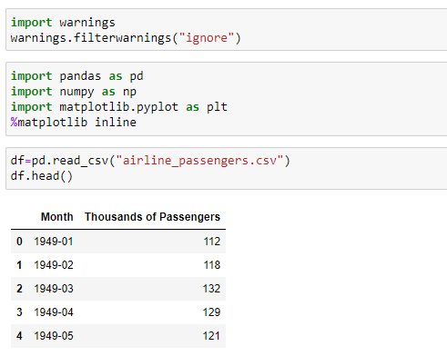
Read the dataset (airline_passengers.csv) with the help of the read_csv method from the Pandas package and display the first 5 rows using the head method.

Code:

df=pd.read_csv(“airline_passengers.csv”)
df.head()

Explore The Data

Explore the dataset with help of the built-in methods of the Pandas package.

Code:

df.info()df.describe()

As we can see the month column is in the form of object format. We need to convert it into the date-time format by using the to_datetime method and then assign it as the index of the data frame using the set_index method.

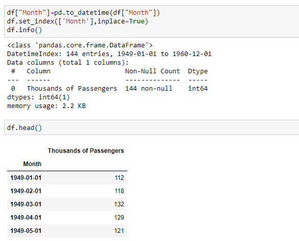
Here, the inplace value is True means the data frame itself gets modified based on the operation applied.

Set the frequency of the date-time index to “MS” using the freq attribute because the dates of the index are at the beginning of the month.

Code:

df.index.freq = ‘MS’

Check For Null Values

Let's check whether the data frame contains null values or not by using the isnull method.

Code:

df.isnull().sum()

No null values are present in the dataset. Otherwise, we would use some techniques to handle missing values like forward-filling, backward-filling, interpolation, etc.

Plot The Data

Plot the data frame using the plot method from the matplotlib library to see how data behaves through time. Here, the figure method is used to set the parameters of the plot.

Code:

plt.figure(figsize=(12,6))
plt.plot(df[‘Thousands of Passengers’])
plt.title(“Monthly total of Airline Passengers”)
plt.ylabel(“In Thousands”)
plt.xlabel(“year”)
plt.show()

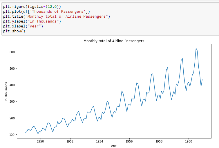
From the above image, we can say that the data is having an upward trend which means a gradual increment of values through time and there is some seasonality in the graph.

Check For Seasonality

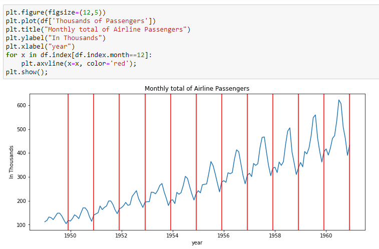
Seasonality is a pattern of data in which the data varies at regular intervals every year. It can be on a weekly, monthly & quarterly basis. In order to understand it clearly, divide the plot based on seasonality. Here, we can say that it is on yearly basis from the above figure.

Code:

plt.figure(figsize=(12,5))
plt.plot(df[‘Thousands of Passengers’])
plt.title(“Monthly total of Airline Passengers”)
plt.ylabel(“In Thousands”)
plt.xlabel(“year”)
for x in df.index[df.index.month==12]:
 plt.axvline(x=x, color=’red’);
plt.show();

Decompose The Signal ( Data )

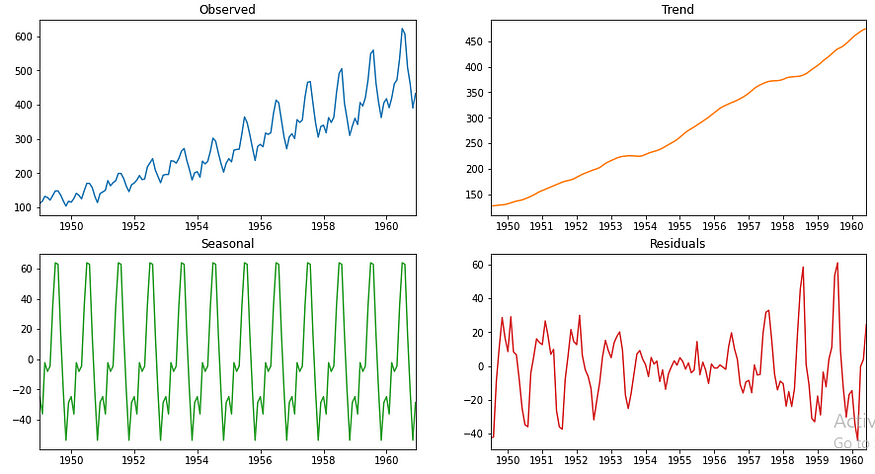
In order to get much clarity, let's decompose the plot into three components(trend, seasonality, residual plots) by using the seasonal_decompose method from the statsmodels library.

Here, the model attribute is given as additive because the graph is gradually increasing with respect to time(trend component). If it increases exponentially then we can assign it as multiplicative.

Code:

from statsmodels.tsa.seasonal import seasonal_decompose
result = seasonal_decompose(df[‘Thousands of Passengers’], model=’additive’)
fig, axs = plt.subplots(2, 2,figsize=(15,8))
axs[0, 0].plot(result.observed)
axs[0, 0].autoscale(axis=’x’,tight=True)
axs[0, 0].set_title(‘Observed’)
axs[0, 1].plot(result.trend,’tab:orange’)
axs[0, 1].autoscale(axis=’x’,tight=True)
axs[0, 1].set_title(‘Trend’)
axs[1, 0].plot(result.seasonal, ‘tab:green’)
axs[1, 0].autoscale(axis=’x’,tight=True)
axs[1, 0].set_title(‘Seasonal’)
axs[1, 1].plot(result.resid, ‘tab:red’)
axs[1, 1].autoscale(axis=’x’,tight=True)
axs[1, 1].set_title(‘Residuals’)
plt.show()

Statistical Test For Stationarity

Let’s do one last step before training the model. That is, check for the stationarity of the data. Stationarity means the data’s mean and variance do not change throughout the x-axis (timestamps). In order to check it, we need to perform a statistical technique that is called Augmented Dickey-Fuller test.

• In this test, if the p-value is less than the significance level (0.05 or 5%) then there is strong evidence against the Null Hypothesis. So, we reject Null Hypothesis and conclude that the data is stationary and has no unit root.
• If the p-value is greater than the significance level (0.05 or 5%) then there is weak evidence against the Null Hypothesis. So, we accept Null Hypothesis and conclude that the data is non-stationary and has a unit root.

Import the adfuller method from the statsmodels library to implement the ADF test. A custom function is defined for the ADF test so that it can be called multiple number times as per our requirement.

Code:

from statsmodels.tsa.stattools import adfuller
def adf_test(df):
 result=adfuller(df)
 print("P Value: ",result[1])
 if result[1]<=0.05:
 print("Strong evidence aganist Null Hypothesis. So, reject Null Hypothesis and conclude data is stationary.")
 return(Tr)
 else:
 print("Weak evidence aganist Null Hypothesis. So, accept Null Hypothesis and conclude data is non-stationary.")
 return(False)
adf_test(df)

If our data is non-stationary, then we need to make it stationary to forecast the future and then apply it to the model. Converting non-stationary data to stationary data can be achieved by differencing the data with its time lag.

Automated Conversion From Non-stationary Data To Stationary Data

Let me define a custom function to automate the conversion of non-stationary data to stationary data and to display the d-value( how many times the data is differenced ).

Code:

def convert_non_stationary_to_stationary(df):
 d=0
 new_df=df
 while True:
 new_df=new_df-new_df.shift()
 new_df.dropna(inplace=True)
 d=d+1
 if adf_test(new_df):
 print("d-value is",d)
 break
convert_non_stationary_to_stationary(df)

Time-series Forecasting Models

Now, select the model based on the data. Before doing it, Let me brief you about each model and its significance.

• Auto Regression—It is the regression of the variable against itself( its lagged versions ). Here, the order of lags is represented by p. We obtain the p-value from the PACF plot.​
• Moving Average — It is dependent on the current observations and the lagged residual errors of the data. Here, the order of lags is represented by q. We obtain the q-value from the ACF plot.​
• ARMA ( AR+MA ) —It is a combination of the Auto Regression model and Moving Average model. It only analyses the stationary time-series data in the form of two polynomial equations without differencing. Its order is defined by ( p,q )components.
• ARIMA ( AR+I+MA ) — It is a combination of the Auto Regression model and Moving Average model. It only analyses the time-series data in the form of two polynomial equations with differencing to convert stationary from non-stationary data. Its order is defined by ( p,d,q ) components.
• SARIMAX (S+AR+I+MA+X) —It is a combination of seasonal components with the ARIMA components and exogenous variables. It is used to forecast seasonal time-series data. Its order is defined by ( p, d, q ) components and seasonal components( P, D, Q ).

Exogenous variable

An exogenous variable is a variable that might affect the variables in the dataset but can not be affected by any other variables.

For example, weather can affect the yield of the crop but vice versa is not possible.

Select The Order Of The Model

Now, the most crucial part forecasting the future. Generally, you might select a model among the models mentioned above and find out p,d,q components from ACF and PACF plots. After that, you would train the model and test it, and forecast the future. Most often, This particular way of following the steps might be messy.

Auto ARIMA Model

Instead of that approach, It’s better to go with an automated approach this can be either using the auto_arima method or using the GridSearchCV method ( hyper-parameter tuning).

Split the data into train and test datasets and fit the dataset to the auto_arima method.

Code:

train = df.iloc[:len(df)-30]
test = df.iloc[len(df)-30:]
from statsmodels.tsa.statespace.sarimax import SARIMAX
from statsmodels.graphics.tsaplots import plot_acf,plot_pacf
from pmdarima import auto_arima
auto_arima(df['Thousands of Passengers'],seasonal=True,m=12).summary()

Observations :

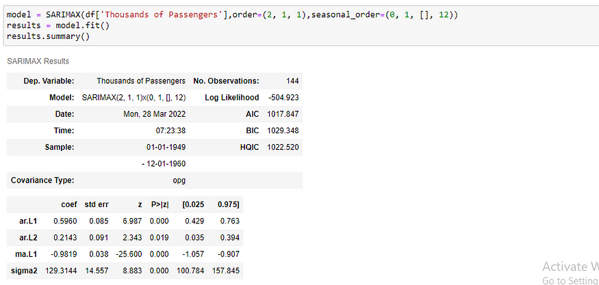
Here m-value is based on seasonality. It is 12 for monthly data, 4 for quarterly data, and 1 for annual data. As we can see from the above picture, the best prediction is done by SARIMAX(2, 1, 1)x(0, 1, [], 12) model.

Fit The Model With Train Dataset

Let’s take the order, implement the model by fitting it with train data and predict it with test data.

Code:

model = SARIMAX(train[‘Thousands of Passengers’],order=(2, 1, 1),seasonal_order=(0, 1, [], 12))
results = model.fit()
results.summary()

Predict The Model With Test Dataset

Code:

start=len(train)
end=len(train)+len(test)-1
predicted_values = results.predict(start=start, end=end)
ax = test[‘Thousands of Passengers’].plot(figsize=(12,5))
predicted_values.plot()
plt.legend()
ax.autoscale(axis=’x’,tight=True)

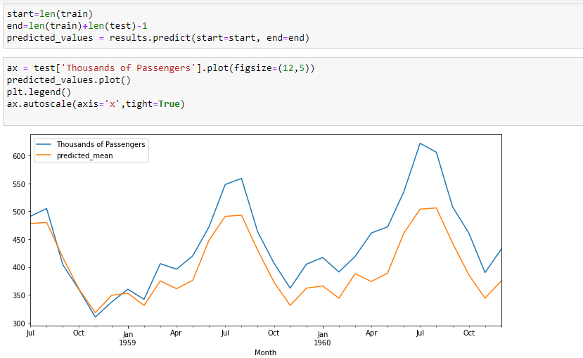
As we can see in the above picture, the model is performing well. It almost fits the data.

Evaluate The Model

Now, evaluate the model with the test dataset and find out the RMSE, MSE, MAE, and MAPE. Import these parameters from the sklearn library.

Code:

import sklearn as sk
from sklearn.metrics import mean_squared_error
from sklearn.metrics import mean_absolute_error
from sklearn.metrics import mean_absolute_percentage_error
print("mean_squared_error :",mean_squared_error(test['Thousands of Passengers'],predicted_values ))
print("root_mean_squared_error :",mean_squared_error(test['Thousands of Passengers'],predicted_values, squared=False))
print("mean_absolute_error :",mean_absolute_error(test['Thousands of Passengers'],predicted_values))
print("mean_absolute_percentage_error :",mean_absolute_percentage_error(test['Thousands of Passengers'],predicted_values))

From the above image, we can see the error values are less. So, we can conclude that our model is performing well for the test data.

Forecast the Future…U+1F60E

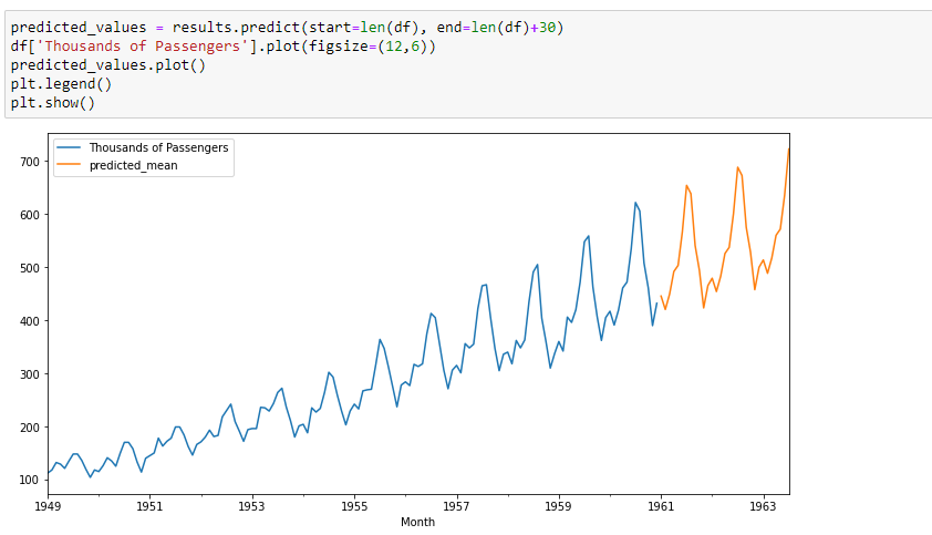
Retrain the model of the same order with the entire data, and forecast the future.

Code:

model = SARIMAX(df['Thousands of Passengers'],order=(2, 1, 1),seasonal_order=(0, 1, [], 12))
results = model.fit()
results.summary()predicted_values = results.predict(start=len(df), end=len(df)+30)
df['Thousands of Passengers'].plot(figsize=(12,6))
predicted_values.plot()
plt.legend()
plt.show()

Source Code

GitHub – balupeddireddy08/Univariate_Time_Series_Analysis

Conclusion

I would like to suggest you follow the same flow to perform the time-series analysis on the data. Hope you enjoy reading the article and is helpful for you… U+1F91DU+1F3FBU+1F91DU+1F3FBU+1F91DU+1F3FB

Let me know if you have any doubts and correct me if anything is wrong with this article. All suggestions are accepted…U+270C️

Happy LearningU+1F60E

Join thousands of data leaders on the AI newsletter. Join over 80,000 subscribers and keep up to date with the latest developments in AI. From research to projects and ideas. If you are building an AI startup, an AI-related product, or a service, we invite you to consider becoming a sponsor.

Published via Towards AI