The Combinatorial Purged Cross-Validation method

Author(s): Berend

Originally published on Towards AI the World’s Leading AI and Technology News and Media Company. If you are building an AI-related product or service, we invite you to consider becoming an AI sponsor. At Towards AI, we help scale AI and technology startups. Let us help you unleash your technology to the masses.

This article is written by Berend Gort & Bruce Yang, core team members of the Open-Source project AI4Finance. This project is an open-source community sharing AI tools for finance and a part of the Columbia University in New York. GitHub link:

AI4Finance Foundation

Colab Notebook

Google Colaboratory

Introduction

This article discusses a robust backtesting method for time series data named the PurgedKFold cross-validation (CV) method. On the internet, limited information is present on the PurgedKFoldCV method. There are existing codes, except their usages are not explained. The idea of PurgedKFoldCV is well described in Lopez de Prado, M. (2018) in Advances in financial machine learning. Therefore, in this article, we will show you how to get your PurgedKFoldCV in a correct manner

Why traditional cross-validation fails

Many papers in the field show promising results on k-fold cross-validation (CV) methods. Their abundance is so great on the internet that more specific methods almost cannot be found any longer.

Maybe you are here now and have read a bunch of literature that the traditional k-fold CV works well. However, it is almost certain that those results are at fault. Reasons:

1. Because observations cannot be expected to be drawn via an IID process, k-fold CV fails in finance.
2. Another cause for CV’s failure is that the testing set is employed several times during the development of a model, resulting in multiple testing and selection bias.

Let us focus on the first part argument. When the training set contains information that appears in the testing set, leakage occurs. Time-series data is often serially correlated, such as crypto Open-High-Low-Close-Volume (OHLCV) data. Consider the following example of a serially correlated characteristic X that is linked to labels Y based on overlapping data:

• Serially correlated observations. That means the following few observations depend on the value of the current observation.
• Target labels are derived from overlapping data points. For example, we have a target label in 10 samples in the future, determining if the price is going down, stays the same, or up. We target label this [0, 1, 2]. This labeling is performed on future values.

Therefore, when we place these data points in different sets, we leak information from one set to the other. Let us prevent this.

• Purging: before a test set, after a train set, remove 10 samples from the train set such that no leakage occurs from the train set to the test set.
• Embargoing: for cases where purging fails to prevent all leakage. After a test set, remove an integer amount of samples from the train set before a train set.

Walk forward back-testing method

The walk-forward (WF) methodology is the most used backtest method in the literature. WF is a historical simulation of the strategy’s performance in the past. Each strategy decision is based on information gathered before the decision was made.

WF enjoys two key advantages:

1. WF has a clear historical interpretation and with comparable performance to paper trading.
2. History is a filtration; therefore, using the endpoint data guarantees that the testing set is completely out-of-sample (OOS).

And three main disadvantages:

1. Just one single scenario is tested, which is easily overfit.
2. WF is not representative of future performance, as results can be biased by the particular sequence of data points (for example, only testing in a significant uptrend).
3. The third disadvantage of WF is that the initial decisions are made on a smaller portion of the total sample.

The Cross-Validation method

Investors often ask how a strategy would perform if subjected to, for example, the 2008 crisis. One way to answer that is to split the observation into training and testing sets, where the training set is outside the 2008 crisis, and the testing set exactly experiences the crisis.

For instance, a classifier might be trained from January 1, 2009, to January 1, 2017, and then evaluated from January 1, 2008, to December 31, 2008. Because the classifier was trained on data that was only accessible after 2008, the performance we would acquire for 2008 is not historically correct. The test’s purpose, however, was not historical accuracy. The goal of the test was to put a 2008-unaware approach through a stressful situation similar to 2008.

The goal of backtesting through cross-validation (CV) is not to derive historically accurate performance but to infer future performance from several out-of-sample (OOS) scenarios. For each period of the backtest, we simulate the performance of a classifier that knew everything except for that period.

That is why Amazon has obsessed with price, selection, and availability from day one and still does today. CV method advantages:

1. The test is not based on a specific (historical) scenario. CV evaluates k different scenarios, only one of which matches the historical sequence.
2. Every judgment is based on equal-sized groups. As a result, outcomes may be compared across periods regarding the amount of data needed to make decisions.
3. Every observation is part of one and only one testing set. There is no warm-up subset, allowing for the most extensive out-of-sample simulation feasible.

CV method disadvantages:

1. A single backtest path is simulated, similar to WF. Per observation, one and only one forecast is generated.
2. CV lacks a solid historical context. The output does not represent how the strategy performed in the past but rather how it could perform in the future under various stress conditions (a helpful result in its own right).
3. Leakage is possible because the training set does not follow the testing set.
4. Avoid leaking testing knowledge into the training set, extreme caution must be exercised

The Combinatorial Purged Cross-Validation Backtesting Algorithm

CPCV provides the exact number of combinations of training/testing sets required to construct a set of backtesting paths while purging training observations that contain leaked information, given a set of backtest paths targeted by the researcher.

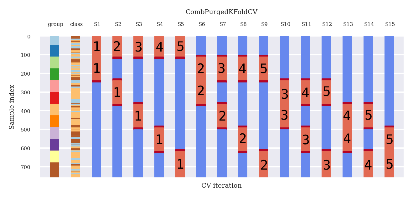
First, we have our data, say 1000 data points. Imagine we want to split those 1000 datapoints into 6 groups. Of these 6 groups, we want 2 test groups (figure below).

How many data splits are possible? That is nCr(6, (6–2) ) = 15. See Figure 1.

Every split involves k=2 tested groups, which means that the total amount of testing groups is k * N_splits, which is 30. Moreover, since we have computed all possible combinations, these tested groups are uniformly distributed across all N. Therefore, there is a total number of paths 30 / 6= 5 paths.

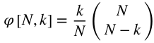
Figure 1 indicates the groups that make up the testing set with an x and leaves the groups that make up the training set unmarked for each split. This train/test split technique allows us to compute 5 backtest pathways because each group is a member of 𝜑[6, 2] = 5 testing sets.

Probably you are a bit confused at this point and have questions like:

1. What models are you training for what split, and why?

First, let us agree on some notation, few examples:

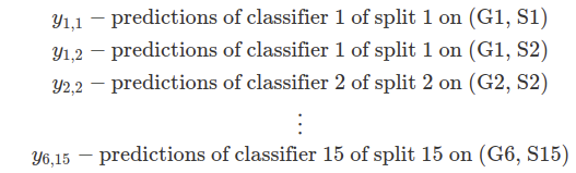
For every vertical split (S1, S2 … S15), train a classifier to determine your target labels y(1,1), y(1,2), etcetera. This classifier base model is consistent for each split, but the predictions it makes are different. Therefore it is still a different classifier!

So a few basic examples (See Figure 1):

• Split 1 || train : (G3, S1), (G4, S1), (G5, S1), (G6, S1) || test : (G1, S1), (G2, S1) || → classifier 1 → predictions y(1,1), y(1,2) on (G1, S1), (G2, S1)
• Split 2|| train : (G2, S2), (G4, S2), (G5, S2), (G6, S2) || test : (G1, S2), (G3, S1) || → classifier 2 → predictions y(1,2), y(3,2) on (G1, S2), (G3, S2)
• …….
• Split 15|| train : (G1, S15), (G2, S15), (G3, S15), (G4, S15) || test : (G5, S15), (G6, S15) || → classifier 15 → predictions y(5,15), y(6,15) on (G5, S15), (G6, S15)

2. Why are these backtest paths unique?

Imagine we have trained our classifiers and computed all of the predictions for all the (x) locations in Figure 1. Therefore, we can now apply our strategy based on these predictions.

Take a look at Figure 2. A path generation algorithm distributed all the predictions on the test groups to one of the 5 unique paths. Recombining the path sections can be done in any manner, and different combinations should converge to the same distribution.

The main point is: that all of these walk-forward paths are purely out-of-sample (OOS). The predictions made by your classifiers have not been trained on these paths! (Figure 2).

Example, path 1:

• Classifier 1 did not train on (G1, S1), (G2, S1), and therefore we can use those predictions to get to our strategy (whatever that may be).
• Classifier 2 did not train on (G3, S2), and therefore we can use those predictions for the next bit of data.
• …..
• Classifier 5 did not train on (G6, S5) and therefore…
• The duplicate accounts for the remainder of the paths

Conclusion: we now have 5 walks forward backtest paths instead of 1. Therefore, 5 Sharpe ratios or whatever metrics you are using to determine your model’s performance. These multiple metrics allow for ‘statistical backtesting’ and make the probability of false discoveries negligible (assuming a large enough number of paths).

PurgedKFoldCV Code

Sam31415 from MIT made a package for this, and after a struggle, we found out how to use it. However, the CombPurgedKFoldCV class required some repairs! So we recommend using my version of it (provided in the Colab).

If you want details, you can look on GitHub for the details below:

GitHub – sam31415/timeseriescv: Scikit-learn style cross-validation classes for time series data

Your data

The data frame on which you are going to apply this has two requirements:

1. It has to be a time series
2. It needs target labels that are produced on future values

That is all; you can do this on any data frame!

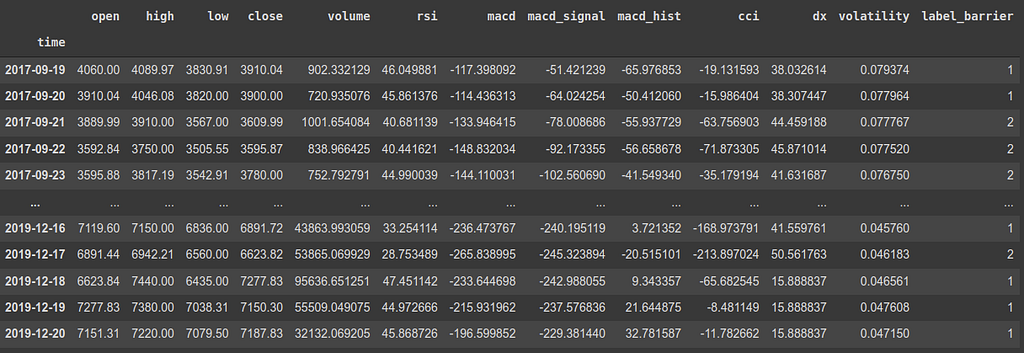
This is an example of a data frame considering the features of Bitcoin. It has a timestamp, some features, and a label_barrier based on t_final in the future. If you want to know more about how we got to this particular example data frame click on the story below:

Crypto feature importance for Deep Reinforcement Learning

The code

Remember, we have observations and evaluations. If you are interested in Combinatorial PurgedKFoldCV, your evaluations are performed in the future and linked to the time of your observations! For example, in my case, my evaluations are +t_final data points in the future.

We need the times of the observations and the evaluations, which can be done as follows. In the snipped below:

1. Select the bitcoin data.
2. Get the index of the Bitcoin data, which are the timestamps (see data frame up).
3. Drop the target variable from the features data frame X (label_barrier), and drop the last t_final features. These are useless as their prediction values are NaN.
4. Select the target variable y, give it the index of the old data frame.
5. Throw away the last t_final predictions (they are NaN as there is no data to predict beyond).
6. Set the times at which the observation was made (prediction times).
7. Set the times at which the prediction of the target variable was made (evaluation times).

Plotting your Combinatorial PurgedKFoldCV

Now we can create an instance of the class CombPurgedKFoldCV. Let us stick to the Lopez example for simplicity, where the groups N=6 (Python from 0, therefore 5!), and the tested groups is k=2.

The embargo depends on your problem, but for simplicity, we take the embargo the same value as the purging.

The back_test_paths_generator function is given and described at the bottom of this article.

# Constants
num_paths = 5
k = 2
N = num_paths + 1
embargo_td = pd.Timedelta(days=1)* t_final

# instance of class
cv = CombPurgedKFoldCV(n_splits=N, n_test_splits=k, embargo_td=embargo_td)

# Compute backtest paths
_, paths, _= back_test_paths_generator(X.shape[0], N, k)

# Plotting
groups = list(range(X.shape[0]))
fig, ax = plt.subplots()
plot_cv_indices(cv, X, y, groups, ax, num_paths, k)
plt.gca().invert_yaxis()

I built the following plotting function based on Sklearns visualization of the cross-validation page, adapted the existing functions and added a few necessary items.

Note that in line 13, the for loop is exactly how it would be during your training process. That is the line you want to copy to be training each classifier eventually!

The results

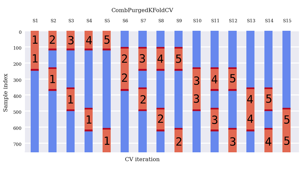
Figure 3 shows the results of the plotting code provided.

In Figure 3:

• Blue: train periods
• Embargo / purged periods: deep red
• Test periods: light red

Now, look at the deep red embargo/purged periods:

• There is a purging period before a testing period AND after a training period.
• After a testing period, we have a purging period and embargoing period
• The embargoing period is larger than the purging period

Thus, there will be a larger gap at the end of a testing set than before the beginning of a testing set.

Now please take some time and compare Figure 3 and Figure 4, and note equality.

Combinatorial PurgedKFoldCV Backtest path generator explained

Using this function is quite easy, and it only takes three arguments (amount of observations, N, and k). The goal is to describe paths 1–5 shown below. Read quickly through it, and below the code, we will explain the result paths from this function.

In the Colab dataset, we have 813 observations. The input size does not matter to explain this function; imagine we only have 30 observations, and still N=6 groups and still k=2 tested_groups.

We have added 1 for simplicity of thinking on the output of the paths in this notebook!

# Compute backtest paths
N_observations = 30 ## colab dataset 813

_, paths, _= back_test_paths_generator(N_observations, N, k, prediction_times, evaluation_times)

# Add plus one to avoid pythonic 0 counting (more logical for you guys)
paths + 1

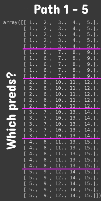
See what this function does? Each column in Figure 6 is a backtest path. In this case, our data spans 30 data points. Therefore the size of each group is 5 data points (with 6 groups). We have indicated the group splits with pink horizontal lines. The numbers indicate which predictions you should be taking (In Figure 3).

For example, for path 4:

• Take predictions for data points 1–5 from classifier 4
• Take predictions for data points 6–10 from classifier 8
• Take predictions for data points 11–15 from classifier 11
• Take predictions for data points 16–20 from classifier 13
• Take predictions for data points 21–25 from classifier 13
• Take predictions for data points 25–25 from classifier 14

That is it!

Conclusion

Traditional time-series backtesting is sample in-efficient, and leakage occurs. Purging and embargoing are necessary to avoid extreme leakage of information. Traditional walk forward backtesting methods only test a single scenario, easily overfit. Also, WF is not representative of future performance, as the particular sequence of data points can bias results. Finally, WF’s initial decisions are based on a small portion of the total sample space. PurgedK-FoldCV solves these problems by performing the backtests on equal-sized groups. Also, every observation is part of one and only one testing set. Finally, Combinatorial PurgedK-FoldCV allows for many unique backtest paths, which reduces the likelihood of false discoveries.

This article provided code and a full explanation of how to index the combinatorial PurgedKFoldCV. The (dis)advantages of the most used method in literature are summarized and compared to the (dis)advantages of the Combinatorial PurgedKFoldCV method. After that, an in-depth look is taken at the method, and several hard-to-grasp points are elaborated. Finally, a small discussion and explanation of the Colab Code are included.

I hope it will have many happy users in the future.

Thanks for getting to the bottom of “best technical indicators for Bitcoin from TA-lib”!

~ Berend & Bruce

Reference

Prado, M. L. de. (2018). Advances in financial machine learning.

---

The Combinatorial Purged Cross-Validation method was originally published in Towards AI on Medium, where people are continuing the conversation by highlighting and responding to this story.

Join thousands of data leaders on the AI newsletter. It’s free, we don’t spam, and we never share your email address. Keep up to date with the latest work in AI. From research to projects and ideas. If you are building an AI startup, an AI-related product, or a service, we invite you to consider becoming a sponsor.

Published via Towards AI