Feature Transformation

Author(s): Parth Gohil

Originally published on Towards AI the World’s Leading AI and Technology News and Media Company. If you are building an AI-related product or service, we invite you to consider becoming an AI sponsor. At Towards AI, we help scale AI and technology startups. Let us help you unleash your technology to the masses.

When and which feature transformation to use according to data.

The life cycle of the Machine Learning model can be broken down into the following steps.

1. Data Collection
2. Data Preprocessing
3. Feature Engineering
4. Feature Selection
5. Model Building
6. Hyper Parameter Tuning
7. Model Deployment

To build a model we have to preprocess data. Feature Transformation is one of the most important tasks in this process. In the dataset, there will be data with different magnitudes most of the time. So to make our predictions better we have to scale down different features to the same range of magnitude or some specific data distribution. because most of the algorithms will give more importance to the features with high volume rather than giving the same importance to all features. This will lead to wrong predictions and faulty models and we don’t want that.

When to use Feature Transformation

1. In algorithms like K-Nearest- Neighbors, SVM, and K-means which are Distance-based algorithms, They will give more weightage to features with large values because the distance is calculated with values of data points to find out similarities between them. If we feed the algorithm unscaled features the prediction will suffer dramatically.
2. Because we are scaling features down, the area of calculations will also be brought down to a smaller range and a little less time will be spent on calculating. Hence faster model training.
3. In the algorithms like linear regression and logistic regression which work upon gradient-descent optimization, Feature scaling becomes crucial because if we feed data with different magnitudes, it will be way too hard to converge to Global Minima. With values of the same range, it becomes less burden for algorithms to learn.

When not to use Feature Transformation

Most of the ensemble method doesn’t require feature scaling because even if we perform feature transformation, the depth of distribution wouldn’t change much. So in such algorithms, there is no need for scaling unless specifically needed.

There are so many types of feature transformation methods, we will talk about the most useful and popular ones.

1. Standardization
2. Min — Max Scaling/ Normalization
3. Robust Scaler
4. Logarithmic Transformation
5. Reciprocal Transformation
6. Square Root Translation
7. Box-Cox Transformation
8. Johnson transformation

1. Standardization

Standardization should be used when the features of the input dataset have large differences between ranges or when they are measured in different measurements units like Height, Weight, Meters, Miles, etc.

We bring all the variables or features to a similar scale. Where the mean is 0 and the Standard Deviation is 1.

In Standardization, we subtract feature values by their mean and then divide by standard deviation which gives exactly standard normal distribution.

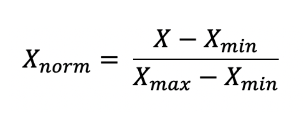
2. Min — Max Scaling / Normalization

In simple terms, min-max scaling brings down feature values to a range of 0 to 1. Until we specify the range we want it to be scaled down to.

In Normalization, we subtract the feature value by its minimum value and then divide it by the range of features (range of feature= maximum value of feature — minimum value of feature).

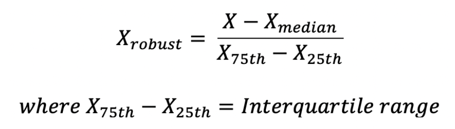
3. Robust Scaler

If the dataset has too many outliers, both Standardization and Normalization can be hard to depend on, in such case you can use Robust Scaler for feature scaling.

You can also say Robust Scaler is robust to outliers 😂.

It scales values using median and interquartile range therefore it doesn’t get affected by very large or very small values of features.

The robust scaler subtracts feature values by their median and then divides by its IQR.

• 25th percentile = 1st quartile
• 50th percentile = 2nd quartile (also called the median)
• 75th percentile = 3rd quartile
• 100th percentile = 4th quartile (also called the maximum)
• IQR= Inter Quartile Range
• IQR= 3rd quartile — 1st quartile

4. Gaussian Transformations

Some Machine Learning algorithms like linear and logistic regression assumes that the data we are feeding them is normally distributed. If the data is normally distributed such algorithms tend to perform better and give higher accuracy. Normalizing a skewed distribution becomes an important part here.

But most of the time data would be skewed so You have to transform it into Gaussian distribution using the following algorithms, you might have to try out a few methods before selecting one since different datasets tend to have different requirements and we can’t fit one method to all the data.

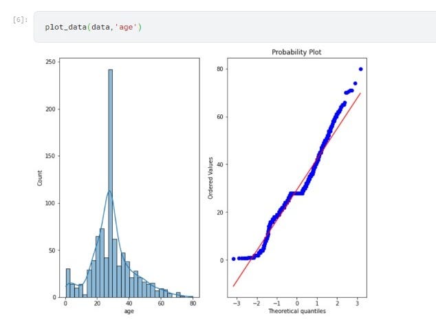
We will use this function to plot data throughout the rest of the article. I will be using the age feature only from the titanic dataset to plot histogram and QQ Plot.

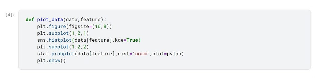
Below the graph is of age feature before feature scaling

A. Logarithmic Transformation

In the Logarithmic Transformation, we will apply log to all values of features using NumPy and store it in the new feature.

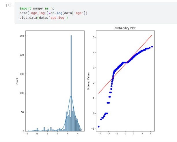
Using Log Transformation doesn’t seem to fit very well in this dataset, it even worsens the distribution by making data left-skewed. So we have to rely on other methods to achieve normal distribution.

B. Reciprocal Transformation

In Reciprocal Transformation, we divide each value of a feature by 1(reciprocal) and store it in the new feature.

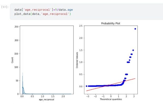
Reciprocal Transformation doesn’t work well with this data, It doesn’t give normal distribution instead it made data even more right-skewed.

C. Square Root Translation

In square root transformation, we raise the values of feature to the power of fraction(1/2) to achieve the square root of a value. We can also use NumPy for this transformation.

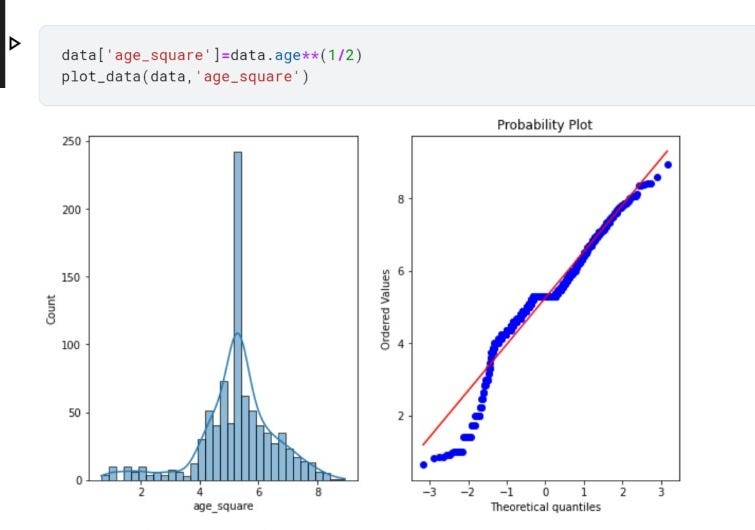
Square root transformation seems to perform better than reciprocal and log transformation with this data but yet it is a bit left-skewed.

D. Box-Cox Transformation

Box-Cox transformation is one of the most useful scaling techniques to transfer data distribution in a normal distribution.

The Box-Cox transformation can be defined as:

T(Y)=(Y exp(λ)−1)/λ

Where Y is the response variable and λ is the transformation parameter. λ varies from -5 to 5. In the transformation, all values of λ are considered and the optimal value for a given variable is selected.

We can calculate box cox transformation using stats from the SciPy module.

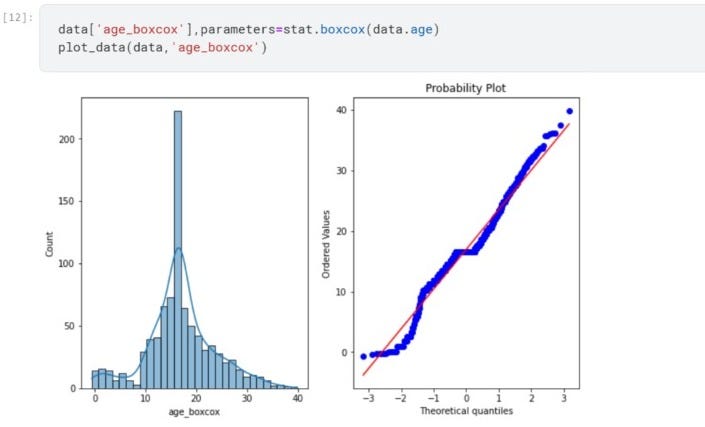
So far box cox transformation seems to be the best fit for the age feature to transform.

Conclusion

There are other techniques also to perform to get Gaussian distribution but most of the time one of these methods seems to fit well on the dataset.

---

Feature Transformation was originally published in Towards AI on Medium, where people are continuing the conversation by highlighting and responding to this story.

Join thousands of data leaders on the AI newsletter. It’s free, we don’t spam, and we never share your email address. Keep up to date with the latest work in AI. From research to projects and ideas. If you are building an AI startup, an AI-related product, or a service, we invite you to consider becoming a sponsor.

Published via Towards AI