Enhancing the Local Details With Adaptive Histogram Equalization
Last Updated on May 22, 2023 by Editorial Team
Author(s): Abhijith S Babu
Originally published on Towards AI.
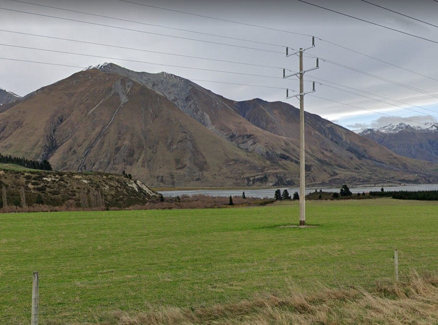
Look at this photo that I took on one of my trips. It is a beautiful mountain.

Now I did some modifications to that image and have a look at it now.

Doesn’t it look better than the original? Well, I did a simple operation on the image called histogram equalization.
Histogram equalization is a widely used image enhancement technology that improves the visual appearance and amplifies the smaller details in the image. It is a technique that maps the pixels into a new set of pixels such that the darkest pixels will be mapped to black while the lightest pixels will be mapped to white.
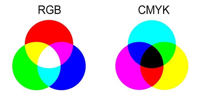
A normal color image consists of three color channels, namely Red, Green, and Blue. Each of the color channels can have an intensity ranging from 0 to 255. All the colors in a digital image can be created by combining each of the color channels with a particular intensity for each channel. For instance, if the intensity of red and green are close to 255 and the intensity of blue is close to zero, we get a color similar to yellow. If all the channels have an intensity of 255, we get white color, while if all channels have an intensity of 0, we will get black color.
For histogram equalization, we divide the input image into three different color channels. Now we can apply histogram equalization on each of the channels. For that, we create a histogram of the image, which represents the frequency of occurrence of each intensity level. From the frequency distribution of the pixels, we will create a cumulative distribution. A cumulative distribution function will say how many pixels have an intensity less than or equal to the given intensity level.
The cumulative distribution created can be normalized to the range [0,1] by dividing each value by the number of pixels in the image. This value can be converted to a scale of [0,255] by multiplying each value by 255. Now we can replace each pixel in the original image with the new corresponding value.
This operation can be done on each color channel, and the output of each color channel can be combined to form a new histogram-equalized image.
Here is a Python code for the same.
from PIL import Image
import matplotlib.pyplot as plt

img = Image.open("path/to/image")
w,h = img.size

# creating histograms of r g and b

pix_r = [0]*255
pix_g = [0]*255
pix_b = [0]*255

for i in range(w):
 for j in range(h):
 r,g,b = img.getpixel((i,j))
 pix_r[r-1] += 1
 pix_g[g-1] += 1
 pix_b[b-1] += 1

plt.subplot(2,1,1)
plt.plot(pix_r,color="red")
plt.plot(pix_g,color="green")
plt.plot(pix_b,color="blue")


#calculating cumulative distribution

for i in range(1,255):
 pix_r[i] += pix_r[i-1]
 pix_g[i] += pix_g[i-1]
 pix_b[i] += pix_b[i-1]

plt.subplot(2,1,2)
plt.plot(pix_r,color="red")
plt.plot(pix_g,color="green")
plt.plot(pix_b,color="blue")
plt.show()

num_pixel = w*h
for i in range(w):
 for j in range(h):
 r,g,b = img.getpixel((i,j))
 new_r = pix_r[r-1]*(255/num_pixel)
 new_g = pix_g[g-1]*(255/num_pixel)
 new_b = pix_b[b-1]*(255/num_pixel)
 img.putpixel((i,j),(int(new_r),int(new_g),int(new_b)))
img.save("equalized_image.jpg")
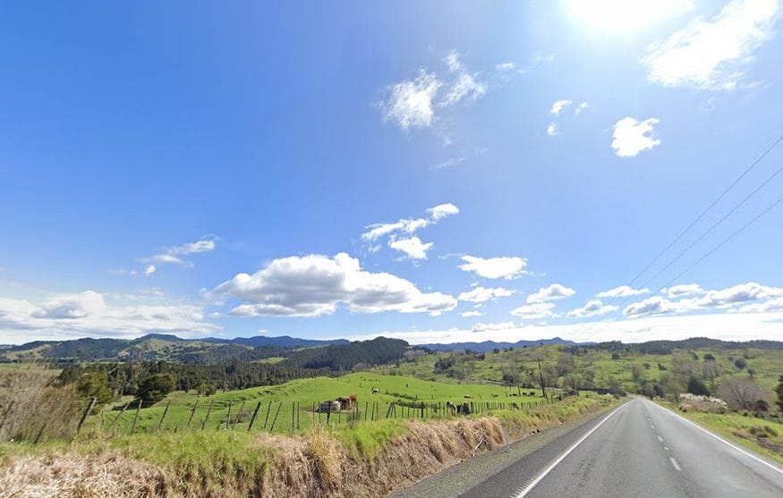
Now consider this image
After histogram equalization, this is the output that I got.
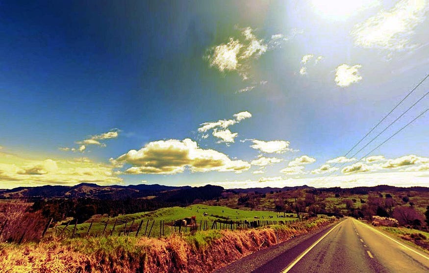
The bottom half of the image got a different tint because of the lighting on the top part of the image. This happened because of the difference in luminescence on the top part and bottom part of the image. What if I equalize each part of the image separately?
This is the output that I got when I divided the image into two blocks and equalized them separately.

Here we can see that the details of the top and bottom parts are enhanced separately. This technique is known as block histogram equalization.
Let us have a look at how block histogram equalization is done.
First, the image is divided into different blocks. Adaptive approaches can be used to divide the image into segments based on edges, textures, and intensities. For this, region growing or segmentation algorithms can be used. Now for each region, histogram equalization is done separately as discussed above. The equalized regions can be combined together to get an enhanced image.
Now, let us have a look at this image, where we do block histogram equalization.


Here we can see the boundary of the segments, which is caused by the intensity discontinuity at the block boundary. This is called a blocking artifact.
To eliminate blocking artifacts, we can use the moving window technique. Here we define an N*N window and apply histogram equalization inside that region, then we slide the window and apply equalization in the new window. This goes on and on until we cover the whole image with the window.
This is a computationally expensive technique but can be used in required situations using clever programming. This technique adaptively enhances the small regions of the image while avoiding blocking artifacts.
There is another efficient approach for removing blocking artifacts. The block histogram equalization can be done on non-overlapping regions as before, but the transfer functions can be smoothly interpolated as we move from one region to another.
Let us see how that is done…
The position of a pixel in a block can be denoted by (s,t) where s is the horizontal position in the block and t is the vertical position in the block. Both s and t are normalized to the range [0,1]. Now we have to identify three neighboring blocks, such that one of them is horizontally closest to the pixel, one vertically closest to the pixel, and one diagonally closest to the pixel.
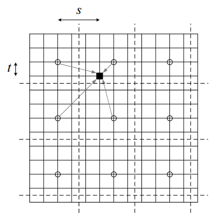
Having the lookup function of all the three blocks we can blend the lookup function of all of these blocks using the equation

In this equation f00 is the lookup function of the block diagonal to the pixel, f10 is the lookup function of the block vertical to the pixel, f01 is the lookup function of the block horizontal to the pixel, f11 is the lookup function of the block containing the pixel.
Using this method, the different blocks are enhanced separately and blended while maintaining a smooth transition between the blocks. This method also reduces the noise amplification problem that is present in other traditional equalization methods. It has to be noted that there are many more variations of adaptive histogram equalization techniques based on the implementation.
I am open to responses if you want to discuss more about histogram equalization.
Join thousands of data leaders on the AI newsletter. Join over 80,000 subscribers and keep up to date with the latest developments in AI. From research to projects and ideas. If you are building an AI startup, an AI-related product, or a service, we invite you to consider becoming a sponsor.
Published via Towards AI
Towards AI Academy
We Build Enterprise-Grade AI. We'll Teach You to Master It Too.
15 engineers. 100,000+ students. Towards AI Academy teaches what actually survives production.
Start free — no commitment:
→ 6-Day Agentic AI Engineering Email Guide — one practical lesson per day
→ Agents Architecture Cheatsheet — 3 years of architecture decisions in 6 pages
Our courses:
→ AI Engineering Certification — 90+ lessons from project selection to deployed product. The most comprehensive practical LLM course out there.
→ Agent Engineering Course — Hands on with production agent architectures, memory, routing, and eval frameworks — built from real enterprise engagements.
→ AI for Work — Understand, evaluate, and apply AI for complex work tasks.
Note: Article content contains the views of the contributing authors and not Towards AI.


