Demystifying Estimation: The Basics

Author(s): Dhruv Gangwani

Originally published on Towards AI the World’s Leading AI and Technology News and Media Company. If you are building an AI-related product or service, we invite you to consider becoming an AI sponsor. At Towards AI, we help scale AI and technology startups. Let us help you unleash your technology to the masses.

Know more about the population

Table of Content

1. Introduction
2. Normal Distribution
3. Central Limit Theorem
4. Need of understanding the basics??
5. Conclusion

Introduction

Statistics is an important foundation of several fields which involves data. There are two major types of statistics:

1. Descriptive statistics: This type of statistics helps to describe, summarize, and visualize data using graphs. Two major elements of descriptive statistics are a measure of central tendency which is all about the central position of the data sample such as mean, median, and mode, and the second one is a measure of variation which is all about the spread of the data sample such as variance and standard deviation. However, it can’t help to make conclusions beyond the data we have.
2. Inferential statistics: Making conclusions about the population is not possible in most cases as it is costly and requires time and resources. For instance, a researcher wants to know the average time a teenager spends studying. Gathering data from every teenager on the planet and making conclusions from it is impossible. So the only way left is to make conclusions about the population from samples. And, this is known as inferential statistics. There are two major elements of inferential statistics:

• Estimation: It involves taking sample parameters into consideration and making conclusions about the parameter of the population. For example, computing the range of values in which the population parameter (In this case, average studying hours of teenagers) falls, If the mean of a sample of randomly selected 10 students is 52.
• Hypothesis Testing: It involves checking the credibility of a claim which is regarding population parameters. For example, the claim by a researcher states that on average a teenager studies for 4 hours a day, and a sample of 10 students is taken whose mean hours of study is 3.2 hours. Then, hypothesis testing helps to check If the claim about the population mean is correct or not.

In this article, We’ll deep dive into the concept of estimation. Before that, I’ll explain a few supporting and foundational concepts which will help you to understand the concept of estimation better

Normal Distribution

There are many possible distributions of data such as skewed, bimodal, uniform etcetera. The normal distribution is a kind of distribution that has the following properties:

1. Bell Shaped
2. Mean, median, and mode are the same and are at the center.
3. Symmetric at Mean
4. It is unimodal i.e. only one mode
5. The total area under the curve is 100%

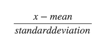
There is a variant of a normal distribution which is known as the Standard normal distribution. It is a kind that has a mean of zero and a standard deviation of 1. Any normal distribution can be transformed to a standard normal distribution using Z scores. Z score is basically a number of the standard deviation a particular value is away from the mean of the data.

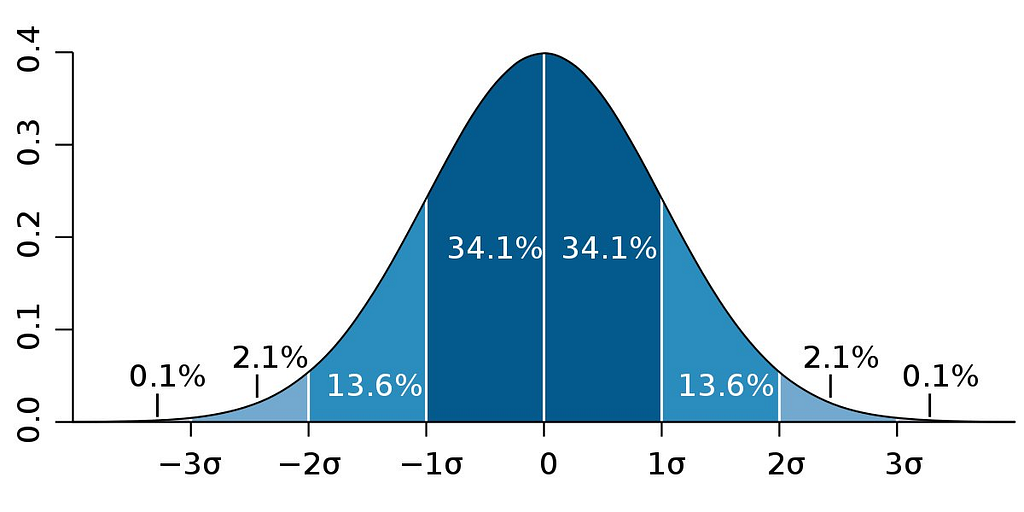
For the normal distribution, the values under the curve are as follows:

• 1 Standard Deviation has 68%
• 2 Standard Deviation has 95%
• 3 Standard Deviation has 99.7%

Central Limit Theorem

Going back to basics beforehand, A sampling distribution of sample means is a distribution using the means computed from all possible random samples of a specific size taken from a population. And, sampling error is the difference between sample parameter and population parameter (for example, the sample mean and population mean) considering the fact that the sample is not a perfect representative of the population.

When all the possible samples of a specific size are extracted from the population without replacement then,

• The mean of the sample means is equal to the population mean.
• The standard deviation of the sample means will be equal to the standard deviation of the population divided by the square root of the sample size.

Central limit theorem states that as the sample size n increases, the shape of distribution of sample means taken from population will approach a normal distribution.

The central limit theorem is important as it is the foundation of two major elements of inferential statistics which are estimation and hypothesis testing. The central limit theorem can be used to answer questions related to the sample mean. There are two conditions:

1. If the population is normal distribution then the distribution of the sample mean will be the normal distribution for any sample size.
2. If the population is not normally distributed, the sample size must be greater than 30.

Looking at the bigger picture, it can be concluded that 68% of the sample means lie within 1 standard deviation from the population mean. Similarly, 95% and 99.7% sample mean lies within 2 and 3 standard deviations from the population mean. To find the exact number of standard deviation, a sample mean is away from the population mean, the Z score is computed,

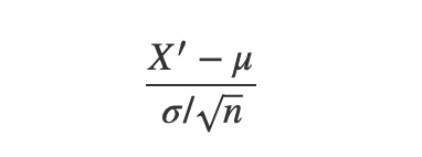
Here, X’ is the sample mean, mu is the mean of sample means, and sigma is the standard deviation of sample means. It is the same as the previous formula of z score but just with the respect to sampling distribution.

Need of understanding the basics??

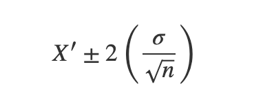
As we learned, Estimation is all about finding the population parameter taking the sample into consideration, and as mentioned above, in sampling distribution and central limit theorem, any sample mean is at X standard deviation of the population mean. For example, 95% of the sample means fall within 2 standard deviations from the population mean, then a sample mean X’ falls within,

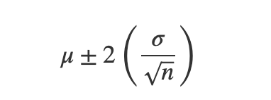
Inversing the formula above, for any X’, 95% probability that the interval mentioned below contains the population mean,

This relation is used to find the interval estimate of the population mean and can only be understood by knowing the basics beforehand.

Conclusion

In this article, we learned foundation concepts for understanding estimation. This is part I of the estimation series. I will post a few other articles that will explain about types of estimation and tests to conduct them.

That’s all folks. I hope you liked it!!

---

Demystifying Estimation: The Basics was originally published in Towards AI on Medium, where people are continuing the conversation by highlighting and responding to this story.

Join thousands of data leaders on the AI newsletter. It’s free, we don’t spam, and we never share your email address. Keep up to date with the latest work in AI. From research to projects and ideas. If you are building an AI startup, an AI-related product, or a service, we invite you to consider becoming a sponsor.

Published via Towards AI