Deep Learning from Scratch in Modern C++: Convolutions
Last Updated on July 25, 2023 by Editorial Team
Author(s): Luiz doleron
Originally published on Towards AI.
Let’s have fun by implementing 2D Convolution in C++.

In the previous story, we covered some of the most relevant coding aspects of machine learning such as functional programming, vectorization, and linear algebra programming.
Now, let’s start our path by actually coding deep learning models with the 2D Convolution implementation. Let’s get it started.
About this series
In this series, we will learn how to code the must-to-know deep learning algorithms such as convolutions, backpropagation, activation functions, optimizers, deep neural networks, and so on using only plain and modern C++.

This story is: Coding 2D convolutions in C++
Check other stories:
0 — Fundamentals of deep learning programming in Modern C++
2 — Cost Functions using Lambdas
3 — Implementing Gradient Descent
… more to come.
Convolutions
Convolution is an old friend from the field of Signal Processing. Originally, it is defined as follows:

In machine learning terminology:
- I(…) is usually referred as Input
- K(…) as Kernel, and
- F(…) as the Feature Map of I(x) given K.
Considering a multi-dimensional discrete domain, we can convert the integral into the following summation:

Finally, for a 2D digital image, we can rewrite it as:

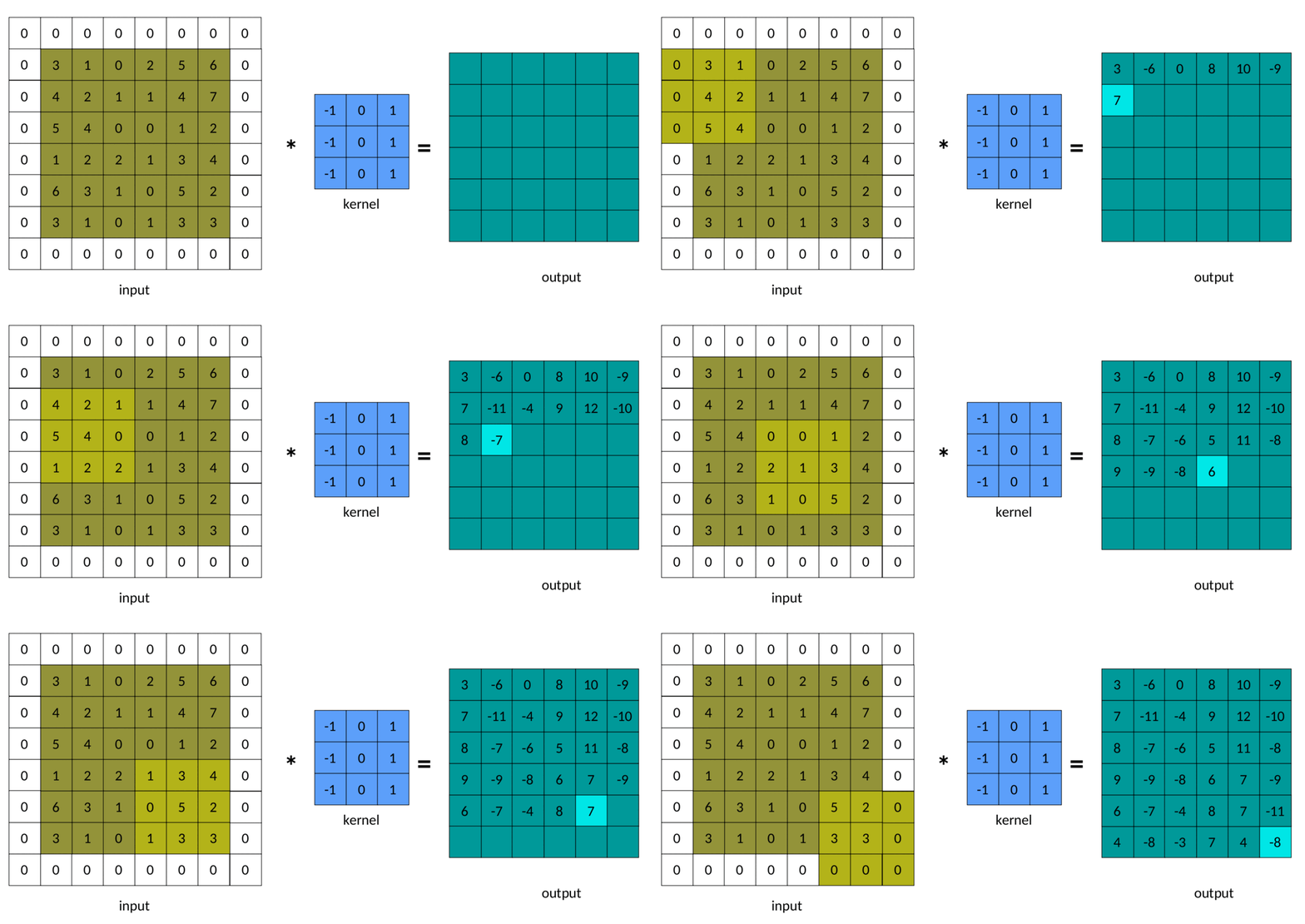
An easier way to understand convolution is by the following illustration:

We can easily see that the kernel slides over the input matrix, generating another matrix as output. This is the simpler case of convolution, called valid convolution. In this case, the dimension of the matrix Output is given by:
dim(Output) = (m-k+1, n-k+1)
where :
mandnare respectively the number of lines and columns in the input matrix andkis the size of the squared kernel.
Now, let’s code our first 2D convolution.
Coding 2D convolution using loops
The most intuitive way to implement a convolution is by using loops:
auto Convolution2D = [](const Matrix &input, const Matrix &kernel)
{
 const int kernel_rows = kernel.rows();
 const int kernel_cols = kernel.cols();
 const int rows = (input.rows() - kernel_rows) + 1;
 const int cols = (input.cols() - kernel_cols) + 1;

 Matrix result = Matrix::Zero(rows, cols);

 for (int i = 0; i < rows; ++i)
 {
 for (int j = 0; j < cols; ++j)
 {
 double sum = input.block(i, j, kernel_rows, kernel_cols).cwiseProduct(kernel).sum();
 result(i, j) = sum;
 }
 }

 return result;
};
There is no secret here. We slide the kernel over columns and lines, applying the inner product for each step. Now, we can use it as simple as:
#include <iostream>
#include <Eigen/Core>

using Matrix = Eigen::MatrixXd;

auto Convolution2D = ...;

int main(int, char **)
{
 Matrix kernel(3, 3);
 kernel <<
 -1, 0, 1,
 -1, 0, 1,
 -1, 0, 1;

 std::cout << "Kernel:\n" << kernel << "\n\n";

 Matrix input(6, 6);
 input << 3, 1, 0, 2, 5, 6,
 4, 2, 1, 1, 4, 7,
 5, 4, 0, 0, 1, 2,
 1, 2, 2, 1, 3, 4,
 6, 3, 1, 0, 5, 2,
 3, 1, 0, 1, 3, 3;

 std::cout << "Input:\n" << input << "\n\n";

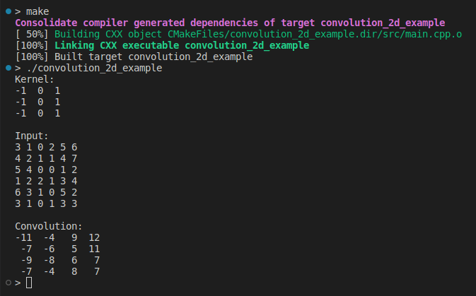
 auto output = Convolution2D(input, kernel);
 std::cout << "Convolution:\n" << output << "\n";

 return 0;
}

This is our very first implementation of convolution 2D designed to be easy to understand. For a while, we are not concerned with performance or input validation. Let’s keep moving to get more insight.
In forthcoming stories, we will learn how to use Fast Fourier Transform and Toeplitz Matrix to implement convolutions.
Padding
In our previous example, we noted that the output matrix is always smaller than the input matrix. Sometimes, this reduction is good, and sometimes it is bad. We can avoid this reduction by adding padding around the input matrix:

The result of padding in convolution can be seen below:

A simple (and brute force) way to implement padded convolutions is as follows:
auto Convolution2D = [](const Matrix &input, const Matrix &kernel, int padding)
{
 int kernel_rows = kernel.rows();
 int kernel_cols = kernel.cols();
 int rows = input.rows() - kernel_rows + 2*padding + 1;
 int cols = input.cols() - kernel_cols + 2*padding + 1;

 Matrix padded = Matrix::Zero(input.rows() + 2*padding, input.cols() + 2*padding);
 padded.block(padding, padding, input.rows(), input.cols()) = input;

 Matrix result = Matrix::Zero(rows, cols);

 for(int i = 0; i < rows; ++i)
 {
 for(int j = 0; j < cols; ++j)
 {
 double sum = padded.block(i, j, kernel_rows, kernel_cols).cwiseProduct(kernel).sum();
 result(i, j) = sum;
 }
 }

 return result;
};
This code is straightforward but very costly in terms of memory usage. Note that we are making a full copy of the input matrix to create a padded version:
Matrix padded = Matrix::Zero(input.rows() + 2*padding, input.cols() + 2*padding);
padded.block(padding, padding, input.rows(), input.cols()) = input;
A better solution can use pointers to control the slice and kernel boundaries:
auto Convolution2D_v2 = [](const Matrix &input, const Matrix &kernel, int padding)
{
 const int input_rows = input.rows();
 const int input_cols = input.cols();
 const int kernel_rows = kernel.rows();
 const int kernel_cols = kernel.cols();

 if (input_rows < kernel_rows) throw std::invalid_argument("The input has less rows than the kernel");
 if (input_cols < kernel_cols) throw std::invalid_argument("The input has less columns than the kernel");

 const int rows = input_rows - kernel_rows + 2*padding + 1;
 const int cols = input_cols - kernel_cols + 2*padding + 1;

 Matrix result = Matrix::Zero(rows, cols);

 auto fit_dims = [&padding](int pos, int k, int length)
 {
 int input = pos - padding;
 int kernel = 0;
 int size = k;
 if (input < 0)
 {
 kernel = -input;
 size += input;
 input = 0;
 }
 if (input + size > length)
 {
 size = length - input;
 }
 return std::make_tuple(input, kernel, size);
 };

 for(int i = 0; i < rows; ++i)
 {
 const auto [input_i, kernel_i, size_i] = fit_dims(i, kernel_rows, input_rows);
 for(int j = 0; size_i > 0 && j < cols; ++j)
 {
 const auto [input_j, kernel_j, size_j] = fit_dims(j, kernel_cols, input_cols);
 if (size_j > 0)
 {
 auto input_tile = input.block(input_i, input_j, size_i, size_j);
 auto input_kernel = kernel.block(kernel_i, kernel_j, size_i, size_j);
 result(i, j) = input_tile.cwiseProduct(input_kernel).sum();
 }
 }
 }
 return result;
};
This new code is much better because here we are not allocating a temporary memory to hold the padded input. However, it can still be improved. The calls input.block(…) and kernel.block(…) are also memory costly.
One solution to
block(…)calls is replacing them using CwiseNullaryOp.
We can run our padded convolution by:
#include <iostream>

#include <Eigen/Core>
using Matrix = Eigen::MatrixXd;
auto Convolution2D = ...; // or Convolution2D_v2

int main(int, char **)
{
 Matrix kernel(3, 3);
 kernel <<
 -1, 0, 1,
 -1, 0, 1,
 -1, 0, 1;
 std::cout << "Kernel:\n" << kernel << "\n\n";

 Matrix input(6, 6);
 input <<
 3, 1, 0, 2, 5, 6,
 4, 2, 1, 1, 4, 7,
 5, 4, 0, 0, 1, 2,
 1, 2, 2, 1, 3, 4,
 6, 3, 1, 0, 5, 2,
 3, 1, 0, 1, 3, 3;
 std::cout << "Input:\n" << input << "\n\n";

 const int padding = 1;
 auto output = Convolution2D(input, kernel, padding);
 std::cout << "Convolution:\n" << output << "\n";

 return 0;
}

Note that, now, the input and output matrices have the same dimensions. For this reason, it is called same padding. The default padding mode, i.e., no padding, is usually called valid padding. Our code allows same , valid or any non-negative padding.
Kernels
In deep learning models, kernels are usually odd-squared matrices such as 3x3 , 5x5 , 11x11 etc. Some kernels are very well-known like Sobel’s filters:

It is easier to see the effect of each Sobel filter on an image:

The code to use Sobel’s filters is here.
Gy highlights the horizontal edges and Gx highlights the vertical edges. For this reason, Sobel kernels Gx and Gy are usually called “edge detectors”.
Edges are primitive features of images such as textures, brightness, colors, etc. The key point of modern computer vision is using algorithms to automatically find kernels such as Sobel filters directly from data. Or, using better terminology, fitting kernels by an iterative training process.
It turns out that the training process teaches computer programs to realize how to perform complex tasks such as recognizing and detecting objects, understanding natural language, etc… The training of kernels will be covered in the next story.
Conclusion and Next Steps
In this story, we wrote our first 2D Convolution and used the Sobel filter as an illustrative case of applying this convolution to an image. Convolutions play a core role in deep learning. They are massively used in every real-world machine learning model today. We shall revisit convolutions to learn how to improve our implementation and also cover some features like strides.
In the next story, we will talk about the most central concern in machine learning: cost functions.
Acknowledgment
I would like to thank Andrew Johnson (andrew@, subarctic.org, https://github.com/andrew-johnson-4) for reviewing this text.
References
A guide to convolution arithmetic for deep learning
The Deep Learning Book, Goodfellow
Neural Networks and Deep Learning: A Textbook, Aggarwal
Computer Vision: Algorithms and Applications, Szeliski.
Join thousands of data leaders on the AI newsletter. Join over 80,000 subscribers and keep up to date with the latest developments in AI. From research to projects and ideas. If you are building an AI startup, an AI-related product, or a service, we invite you to consider becoming a sponsor.
Published via Towards AI
Towards AI Academy
We Build Enterprise-Grade AI. We'll Teach You to Master It Too.
15 engineers. 100,000+ students. Towards AI Academy teaches what actually survives production.
Start free — no commitment:
→ 6-Day Agentic AI Engineering Email Guide — one practical lesson per day
→ Agents Architecture Cheatsheet — 3 years of architecture decisions in 6 pages
Our courses:
→ AI Engineering Certification — 90+ lessons from project selection to deployed product. The most comprehensive practical LLM course out there.
→ Agent Engineering Course — Hands on with production agent architectures, memory, routing, and eval frameworks — built from real enterprise engagements.
→ AI for Work — Understand, evaluate, and apply AI for complex work tasks.
Note: Article content contains the views of the contributing authors and not Towards AI.


