Deep Learning from Scratch in Modern C++
Last Updated on July 25, 2023 by Editorial Team
Author(s): Luiz doleron
Originally published on Towards AI.
Let’s have fun by implementing Deep Learning models in C++.

It is needless to say how relevant machine learning frameworks are for research and industry. Due to their extensibility and flexibility, it is rare to find a project nowadays not using Google TensorFlow or Meta PyTorch.
That said, it may seem counter-intuitive to spend time coding machine learning algorithms from scratch, i.e., without any base framework. However, it is not. Coding the algorithms ourselves provides a clear and solid understanding of how the algorithms work and what the models are really doing.
In this series, we will learn how to code the must-to-know deep learning algorithms such as convolutions, backpropagation, activation functions, optimizers, deep neural networks, and so on, using only plain and modern C++.

We will begin our journey in this story by learning some of the modern C++ language features and relevant programming details to code deep learning and machine learning models.
Check other stories:
1 — Coding 2D convolutions in C++
2 — Cost Functions using Lambdas
3 — Implementing Gradient Descent
… more to come.
What I cannot create, I do not understand. — Richard Feynman
Modern C++, <algorithm>, and <numeric> headers
Once an old language, C++ has drastically evolved in the last decade. One of the main changes is the support of Functional Programming. However, several other improvements were introduced, helping us to develop better, faster, and safer machine learning code.
For the sake of our mission here, C++ included a handy set of common routines in the <numeric> and <algorithm> headers. As an illustrative example, we can obtain the inner product of two vectors by:
#include <numeric>
#include <iostream>

int main()
{
 std::vector<double> X {1., 2., 3., 4., 5., 6.};
 std::vector<double> Y {1., 1., 0., 1., 0., 1.};

 auto result = std::inner_product(X.begin(), X.end(), Y.begin(), 0.0);
 std::cout << "Inner product of X and Y is " << result << '\n';
 return 0;
}

and use functions like accumulate and reduce as follows:
std::vector<double> V {1., 2., 3., 4., 5.};

double sum = std::accumulate(V.begin(), V.end(), 0.0);

std::cout << "Summation of V is " << sum << '\n';

double product = std::accumulate(V.begin(), V.end(), 1.0, std::multiplies<double>());

std::cout << "Productory of V is " << product << '\n';

double reduction = std::reduce(V.begin(), V.end(), 1.0, std::multiplies<double>());

std::cout << "Reduction of V is " << reduction << '\n';

The algorithm header is plenty of useful routines, such as std::transform,std::for_each, std::count, std::unique, std::sort, and so on. Let’s see an illustrative example:
#include <algorithm>
#include <iostream>

double square(double x) {return x * x;}

int main()
{
 std::vector<double> X {1., 2., 3., 4., 5., 6.};
 std::vector<double> Y(X.size(), 0);

 std::transform(X.begin(), X.end(), Y.begin(), square);
 std::for_each(Y.begin(), Y.end(), [](double y){std::cout << y << " ";});
 std::cout << "\n";

 return 0;
}

It turns out that, in modern C++, instead of explicitly using for or while loops, we can rather use functions such as std::transform, std::for_each, std::generate_n, etc., passing functors, lambdas, or even vanilla functions as parameters.
The examples above can be found in this repository on GitHub.
By the way,[](double v){...} is a lambda. Let’s talk about functional programming and lambdas now.
Functional programming
C++ is a multi-paradigm programming language, meaning that we can use it to create programs using different “styles” such as OOP, procedural, and recently, functional.
The C++ support for functional programming begins in the <functional> header:
#include <algorithm> // std::for_each
#include <functional> // std::less, std::less_equal, std::greater, std::greater_equal
#include <iostream> // std::cout

int main()
{

 std::vector<std::function<bool(double, double)>> comparators
 {
 std::less<double>(),
 std::less_equal<double>(),
 std::greater<double>(),
 std::greater_equal<double>()
 };

 double x = 10.;
 double y = 10.;
 auto compare = [&x, &y](const std::function<bool(double, double)> &comparator)
 {
 bool b = comparator(x, y);
 std::cout << (b?"TRUE": "FALSE") << "\n";
 };

 std::for_each(comparators.begin(), comparators.end(), compare);

 return 0;
}

Here, we use std::function, std::less, std::less_equal, std::greater, andstd::greater_equal as an example of polymorphic calls in action without using pointers.
As we already discussed, C++ 11 includes changes in the core of the language to support functional programming. So far, we have seen one of them:
auto compare = [&x, &y](const std::function<bool(double, double)> &comparator)
{
 bool b = comparator(x, y);
 std::cout << (b?"TRUE": "FALSE") << "\n";
};
This code defines a lambda and a lambda defines a function object, that is, an invocable object.
Note that
compareis not the lambda name but the name of a variable to which the lambda is assigned. Indeed, lambdas are anonymous objects.
This lambda consists of 3 clauses: a capture list ([&x, &y] ), a parameter list (const std::function<boll(double, double)> &comparator), and the body (the code between the curly braces{...}).
The parameter list and body clauses work like in any regular function. The capture clause specifies the set of external variables addressable in the lambda’s body.
Lambdas are highly useful. We can declare and pass them like old-style functors. For example, we can define an L2 regularization lambda:
auto L2 = [](const std::vector<double> &V)
{
 double p = 0.01;
 return std::inner_product(V.begin(), V.end(), V.begin(), 0.0) * p;
};
and pass it back to our layer as a parameter:
auto layer = new Layer::Dense();
layer.set_regularization(L2)
By default, lambdas do not cause side effects, i.e., they cannot change the state of objects in the outer memory space. However, we can define a mutable lambda if we want. Consider the following implementation of Momentum:
#include <algorithm>
#include <iostream>

using vector = std::vector<double>;

int main()
{

 auto momentum_optimizer = [V = vector()](const vector &gradient) mutable
 {
 if (V.empty()) V.resize(gradient.size(), 0.);
 std::transform(V.begin(), V.end(), gradient.begin(), V.begin(), [](double v, double dx)
 {
 double beta = 0.7;
 return v = beta * v + dx;
 });
 return V;
 };

 auto print = [](double d) { std::cout << d << " "; };

 const vector current_grads {1., 0., 1., 1., 0., 1.};
 for (int i = 0; i < 3; ++i)
 {
 vector weight_update = momentum_optimizer(current_grads);
 std::for_each(weight_update.begin(), weight_update.end(), print);
 std::cout << "\n";
 }

 return 0;
}

Each momentum_optimizer(current_grads) call results in a different value even though we are passing the same value as the parameter. This happens because we defined the lambda using the keyword mutable.
For our purpose now, the functional programming paradigm is particularly valuable. By using functional features, we will write less but more robust code, performing more complex tasks way faster.
Matrix & Linear Algebra Library
Well, when I said “pure C++”, it was not entirely true. We will be using a reliable linear algebra library to implement our algorithms.
Matrices and tensors are the building blocks of machine learning algorithms. There is no built-in matrix implementation in C++ (and there shouldn’t be one). Fortunately, there are several mature and excellent linear algebra libraries available, such as Eigen and Armadillo.
I have been using Eigen happily for years. Eigen (under the Mozilla Public License 2.0) is header-only and does not depend on any third-party libraries. Therefore, I will use Eigen as the linear algebra backend for this story and beyond.
Common Matrix Operations
The most important matrix operation is matrix-by-matrix multiplication:
#include <iostream>
#include <Eigen/Dense>

int main(int, char **)
{
 Eigen::MatrixXd A(2, 2);
 A(0, 0) = 2.;
 A(1, 0) = -2.;
 A(0, 1) = 3.;
 A(1, 1) = 1.;

 Eigen::MatrixXd B(2, 3);
 B(0, 0) = 1.;
 B(1, 0) = 1.;
 B(0, 1) = 2.;
 B(1, 1) = 2.;
 B(0, 2) = -1.;
 B(1, 2) = 1.;

 auto C = A * B;

 std::cout << "A:\n" << A << std::endl;
 std::cout << "B:\n" << B << std::endl;
 std::cout << "C:\n" << C << std::endl;

 return 0;
}

Usually referred to as mulmat, this operation has a computational complexity of O(N³). Since mulmat is used extensively in machine learning, our algorithms are strongly affected by the size of our matrices.
Let’s talk about another type of matrix-by-matrix multiplication. Sometimes, we need only a coefficient-wise matrix multiplication:
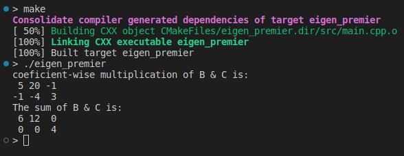
auto D = B.cwiseProduct(C);
std::cout << "coefficient-wise multiplication is:\n" << D << std::endl;
Of course, in coefficient-wise multiplication, the dimension of arguments must match. In the same way, we can add or subtract matrices:
auto E = B + C;
std::cout << "The sum of B & C is:\n" << E << std::endl;

Finally, let’s discuss three very important matrix operations: transpose, inverse , and determinant :
std::cout << "The transpose of B is:\n" << B.transpose() << std::endl;
std::cout << "The A inverse is:\n" << A.inverse() << std::endl;
std::cout << "The determinant of A is:\n" << A.determinant() << std::endl;

Inverses, transposes, and determinants are fundamental to implementing our models. Another key point is to apply a function to each element of a matrix:
auto my_func = [](double x){return x * x;};
std::cout << A.unaryExpr(my_func) << std::endl;

The examples above can be found here.
One word about vectorization
Modern compilers and computer architectures provide an enhanced feature called vectorization. In simple words, vectorization allows independent arithmetic operations to be executed in parallel, using multiple registers. For example, the following for-loop:
for (int i = 0; i < 1024; i++)
{
 A[i] = A[i] + B[i];
}
is silently replaced by the vectorized version:
for(i=0; i < 512; i += 2)
{
 A[i] = A[i] + B[i];
 A[i + 1] = A[i + 1] + B[i + 1];
}
by the compiler. The trick is that the instruction A[i + 1] = A[i + 1] + B[i + 1] runs at the same time as the instruction A[i] = A[i] + B[i]. This is possible because the two instructions are independent of each other, and the underlying hardware has duplicated resources, that is, two execution units.
If the hardware has four executions units, the compiler unrolls the loop in the following way:
for(i=0; i < 256; i += 4)
{
 A[i] = A[i] + B[i] ;
 A[i + 1] = A[i + 1] + B[i + 1];
 A[i + 2] = A[i + 2] + B[i + 2];
 A[i + 3] = A[i + 3] + B[i + 3];
}
This vectorized version makes the program run 4 times faster when compared with the original version. It is noteworthy that this performance gain happens without impacting the original program’s behavior.
Even though vectorization is performed by the compiler, operation system, and hardware under the wood, we have to be attentive when coding to allow vectorization:
- Enabling the vectorization flags required to compile the program
- The loop boundary must be known before the loop starts, dynamically or statically
- The loop body instructions shouldn’t reference a previous state. For example, things like
A[i] = A[i — 1] + B[i]might prevent vectorization because, in some situations, the compiler cannot safely determine ifA[i-1]is valid during the current instruction call. - The loop body should consist of simple and straight-line code.
inlinefunction calls and previously vectorized functions are also allowed. But complex logic, subroutines, nested loops, and function calls in general prevent vectorization from working.
In some circumstances, following these rules is not easy. Given the complexity and code size, sometimes it is hard to say when a specific part of the code was or wasn’t vectorized by the compiler.
As a rule of thumb, the more streamlined and straightforward the code, the more prone to be vectorized it is. Therefore, using standard features of <numeric> , algorithm , functional, and STL containers indicate code that is more likely to be vectorized.
Vectorization in Machine Learning
Vectorization performs an important role in machine learning. For example, batches are often processed in a vectorized way, making a train with large batches run faster than a train using small batches (or no batching).
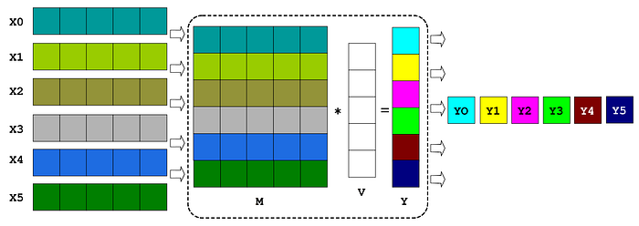
Since our matrix algebra libraries make exhaustive use of vectorization, we usually aggregate the row data into batches to allow faster operation executions. Consider the following example:

Instead of performing 6 inner products between each of the sixXivectors and one Vvector to obtain 6 outputs Y0, Y1, etc, we can stack the input vectors to mount a matrix M with six rows and run it once using a single mulmat multiplication Y = M*V .
The output Y is a vector. We can finally unstack its elements to obtain the desired 6 output values.
Conclusion and Next Steps
This was an introductory talk about how to code deep learning algorithms using modern C++. We covered very important aspects in the development of high-performance machine learning programs such as functional programming, algebra calculus, and vectorization.
Some relevant programming topics of real-world ML projects were not covered here, like GPU programming or distributed training. We shall talk about these subjects in a future story.
In the next story, we shall learn how to code 2D Convolution, the most fundamental operation in deep learning.
Acknowledgment
I would like to thank Andrew Johnson (andrew@, subarctic.org, https://github.com/andrew-johnson-4) for reviewing this text.
References
Intel Vectorization Essentials
Join thousands of data leaders on the AI newsletter. Join over 80,000 subscribers and keep up to date with the latest developments in AI. From research to projects and ideas. If you are building an AI startup, an AI-related product, or a service, we invite you to consider becoming a sponsor.
Published via Towards AI
Towards AI Academy
We Build Enterprise-Grade AI. We'll Teach You to Master It Too.
15 engineers. 100,000+ students. Towards AI Academy teaches what actually survives production.
Start free — no commitment:
→ 6-Day Agentic AI Engineering Email Guide — one practical lesson per day
→ Agents Architecture Cheatsheet — 3 years of architecture decisions in 6 pages
Our courses:
→ AI Engineering Certification — 90+ lessons from project selection to deployed product. The most comprehensive practical LLM course out there.
→ Agent Engineering Course — Hands on with production agent architectures, memory, routing, and eval frameworks — built from real enterprise engagements.
→ AI for Work — Understand, evaluate, and apply AI for complex work tasks.
Note: Article content contains the views of the contributing authors and not Towards AI.


