


")
Data Analysis Project with PandasStep-by-Step Guide (Ted Talks Data)
Last Updated on March 1, 2023 by Editorial Team
Author(s): Fares Sayah
Originally published on Towards AI.
Data Analysis Project with Pandas — Step-by-Step Guide (Ted Talks Data)
Data Analysis Project Guide — Use Pandas power to get valuable information from your data
Table of Contents:
Exploratory Data Analysis is all about answering a specific question. In this post, we will try to answer the following questions:
- Which talks provoke the most online discussion?
- What were the “best” events in TED history to attend?
- Which occupations deliver the funniest TED talks on average?
Read the Data
The first step is to get the data and load it to memory. You can download data from this link: TED Talks. We are using Pandas for data manipulation. Matplotlib, Seaborn, and hvPlot for Data Visualization.
After reading the data successfully, we need to check our data. Pandas have a lot of function that allows us to discover our data effectively and quickly. The goal here is to find out more about the data and become a subject matter expert on the dataset you are working with.
In general, we need to know the following questions:
- What kind of data do we have, and how do we treat different types?
- What’s missing from the data, and how do you deal with it?
- How can you add, change or remove features to get more out of your data?
The Shape of the Data
Use ‘.shape’ to see DataFrame shape: rows, columns
(2550, 17)
Pandas Data Types
To check the types of your data, you can use .dtypes and it will return a pandas series of columns associated with there dtype. Pandas have 7 types in general:
- object, int64, float64, category, and datetime64 are going to be covered in this article.
- bool: True/False values. Can be a NumPy datetime64[ns].
- timedelta[ns]: Differences between two datetimes.
comments               int64
description           object
duration               int64
event                 object
film_date              int64
languages              int64
main_speaker          object
name                  object
num_speaker            int64
published_date         int64
ratings               object
related_talks         object
speaker_occupation    object
tags                  object
title                 object
url                   object
views                  int64
dtype: object
Information About the Data
.info() method prints information about a DataFrame including the index dtype and columns, non-null values, and memory usage.
<class 'pandas.core.frame.DataFrame'>
RangeIndex: 2550 entries, 0 to 2549
Data columns (total 17 columns):
 #   Column              Non-Null Count  Dtype
---  ------              --------------  -----
 0   comments            2550 non-null   int64
 1   description         2550 non-null   object
 2   duration            2550 non-null   int64
 3   event               2550 non-null   object
 4   film_date           2550 non-null   int64
 5   languages           2550 non-null   int64
 6   main_speaker        2550 non-null   object
 7   name                2550 non-null   object
 8   num_speaker         2550 non-null   int64
 9   published_date      2550 non-null   int64
 10  ratings             2550 non-null   object
 11  related_talks       2550 non-null   object
 12  speaker_occupation  2544 non-null   object
 13  tags                2550 non-null   object
 14  title               2550 non-null   object
 15  url                 2550 non-null   object
 16  views               2550 non-null   int64
dtypes: int64(7), object(10)
memory usage: 338.8+ KB
Missing Values
Missing data (or missing values) is defined as the data value that is not stored for a variable in the observation of interest. In Machine Learning, we need to handle missing values. There are many types of missing values:
- Standard Missing Values: These are missing values that Pandas can detect.
- Non-Standard Missing Values: Sometimes it might be the case where there are missing values that have different formats.
- Unexpected Missing Values: For example, if our feature is expected to be a string, but there’s a numeric type, then technically, this is also a missing value.
It’s important to understand these different types of missing data from a statistics point of view. The type of missing data will influence how you deal with filling in the missing values.
- Sometimes you’ll simply want to delete those rows. Other times you’ll replace them.
- A very common way to replace missing values is using a median (for objects) or mean (for numeric values).
But those are weak approaches, some times we need domain knowledge about the data and statistical study to fill in the missing values.
comments              0
description           0
duration              0
event                 0
film_date             0
languages             0
main_speaker          0
name                  0
num_speaker           0
published_date        0
ratings               0
related_talks         0
speaker_occupation    6
tags                  0
title                 0
url                   0
views                 0
dtype: int64
comments              0
description           0
duration              0
event                 0
film_date             0
languages             0
main_speaker          0
name                  0
num_speaker           0
published_date        0
ratings               0
related_talks         0
speaker_occupation    0
tags                  0
title                 0
url                   0
views                 0
dtype: int64
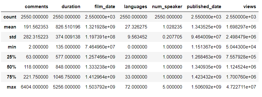
Descriptive Statistics about the Data
.describe() generates descriptive statistics. Descriptive statistics summarize the central tendency, dispersion, and shape of a dataset’s distribution, excluding NaN values.
Analyzes both numeric and object series, as well as DataFrame column sets of mixed data types. The output will vary depending on what is provided. Refer to the notes below for more detail.
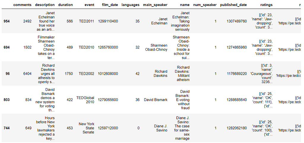
Which talks provoke the most online discussion?
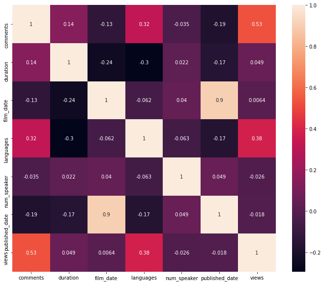
From the heatmap, the number of views correlates well with language and comments.
Limitations of this approach
- Sub comments (nested comments).
- How long has it been online?
To correct this behavior, one solution is to normalize comments by views.
Lessons:
- Consider the limitations and biases of your data when analyzing it
- Make your results understandable
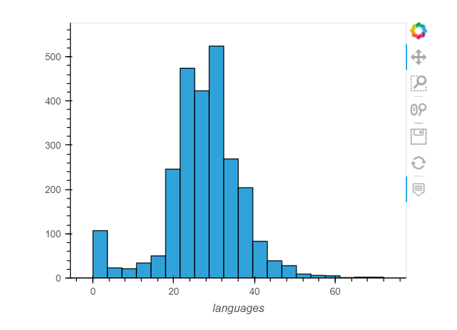
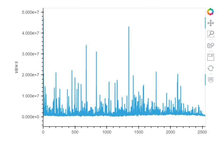
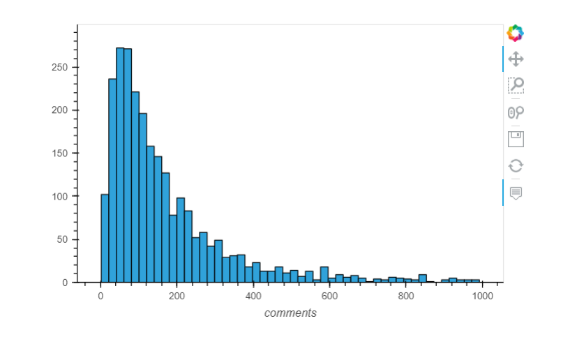
Visualize the distribution of comments
A line plot is not appropriate here (use it to measure something over time)
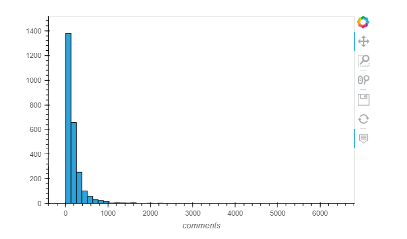
Check how many observations we removed from the plot:
(32, 19)
After filtering the data we lose only a small amount of data. This process is called excluding outliers.
Lessons:
- Choose your plot type based on the question you are answering and the data type(s) you are working with
- Use Pandas one-liners to iterate through plots quickly
- Try modifying the plot defaults
- Creating plots involves decision-making
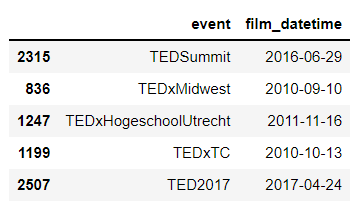
Plot the number of talks that took place each year
The event column does not always include the year
1280    TEDGlobal 2012
163            TED2005
1593    TEDGlobal 2013
2027     TEDWomen 2015
197            TED2008
1286        TEDxAustin
1115      TEDxBrussels
1381          TEDxCHUV
159            TED2007
193            TED2007
Name: event, dtype: object
We can’t rely on event Feature, because most of the events don't have a year:
0    1140825600
1    1140825600
2    1140739200
3    1140912000
4    1140566400
Name: film_date, dtype: int64
Results don’t look right:
0   1970-01-01 00:00:01.140825600
1   1970-01-01 00:00:01.140825600
2   1970-01-01 00:00:01.140739200
3   1970-01-01 00:00:01.140912000
4   1970-01-01 00:00:01.140566400
Name: film_date, dtype: datetime64[ns]
Now the results look right:
0   2006-02-25
1   2006-02-25
2   2006-02-24
3   2006-02-26
4   2006-02-22
Name: film_date, dtype: datetime64[ns]
The new column uses the DateTime datatype (this was an automatic conversion):
comments                       int64
description                   object
duration                       int64
event                         object
film_date                      int64
languages                      int64
main_speaker                  object
name                          object
num_speaker                    int64
published_date                 int64
ratings                       object
related_talks                 object
speaker_occupation            object
tags                          object
title                         object
url                           object
views                          int64
comments_per_view            float64
views_per_comment            float64
film_datetime         datetime64[ns]
dtype: object
DateTime columns have convenient attributes under the dt namespace:
0    2006
1    2006
2    2006
3    2006
4    2006
Name: film_datetime, dtype: int64
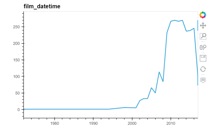
Count the number of talks each year using value_counts():
2013    270
2011    270
2010    267
2012    267
2016    246
2015    239
2014    237
2009    232
2007    114
2017     98
2008     84
2005     66
2006     50
2003     33
2004     33
2002     27
1998      6
2001      5
1984      1
1983      1
1991      1
1994      1
1990      1
1972      1
Name: film_datetime, dtype: int64
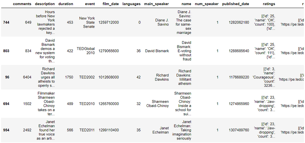
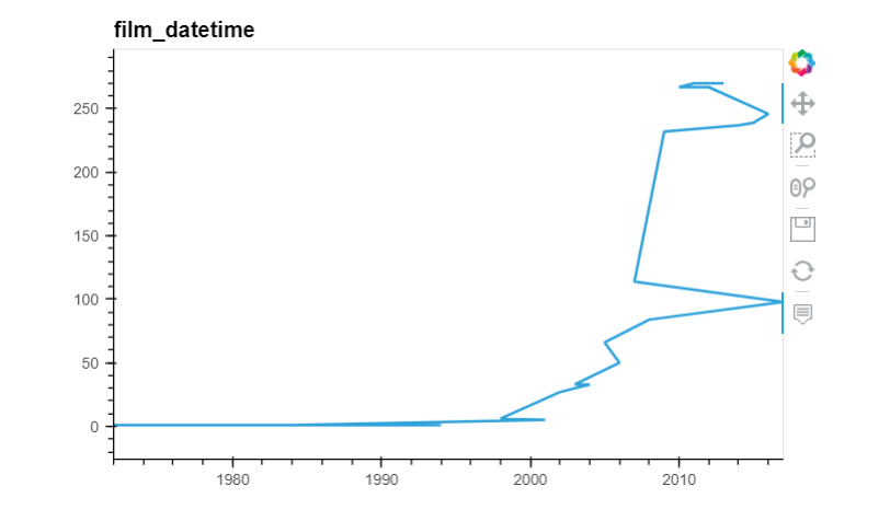
Points are plotted and connected in the order you give them to Pandas:
Need to sort the index before plotting:
Timestamp('2017-08-27 00:00:00')
Lessons:
- Read the documentation
- Use the DateTime data type for dates and times
- Check your work as you go
- Consider excluding data if it might not be relevant
What were the “best” events in TED history to attend?
355
274
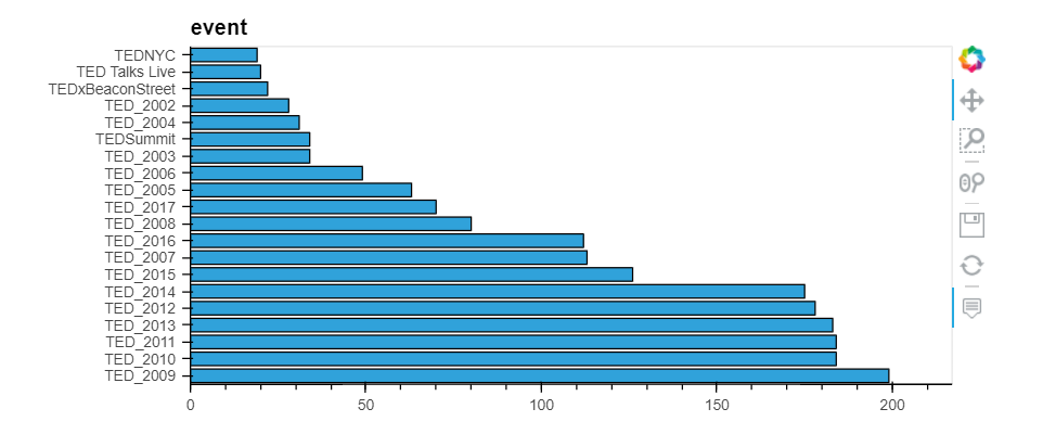
Count the number of talks (great if you value variety, but they may not be great talks):
TED_2009    199
TED_2010    184
TED_2011    184
TED_2013    183
TED_2012    178
Name: event, dtype: int64
Use views as a proxy for “quality of talk”:
event
AORN Congress                  149818.0
Arbejdsglaede Live             971594.0
BBC TV                         521974.0
Bowery Poetry Club             676741.0
Business Innovation Factory    304086.0
Name: views, dtype: float64
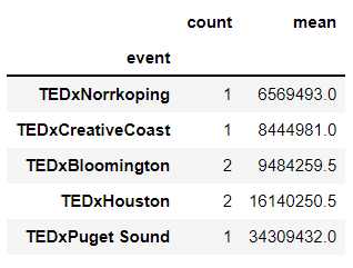
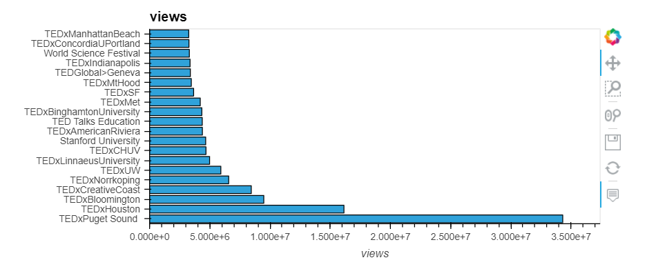
Find the largest values, but we don’t know how many talks are being averaged:
event
TEDxNorrkoping        6569493.0
TEDxCreativeCoast     8444981.0
TEDxBloomington       9484259.5
TEDxHouston          16140250.5
TEDxPuget Sound      34309432.0
Name: views, dtype: float64
Show the number of talks along with the mean (events with the highest means had only 1 or 2 talks):
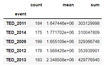
Calculate the total views per event:
Lessons:
- Think creatively about how you can use the data you have to answer your question
- Watch out for small sample sizes
Unpack the rating data
Previously, users could tag talks on the TED website (funny, inspiring, confusing, etc.)
0    [{'id': 7, 'name': 'Funny', 'count': 19645}, {...
1    [{'id': 7, 'name': 'Funny', 'count': 544}, {'i...
2    [{'id': 7, 'name': 'Funny', 'count': 964}, {'i...
3    [{'id': 3, 'name': 'Courageous', 'count': 760}...
4    [{'id': 9, 'name': 'Ingenious', 'count': 3202}...
Name: ratings, dtype: object
Two ways to examine the rating data for the first talk:
"[{'id': 7, 'name': 'Funny', 'count': 19645}, {'id': 1, 'name': 'Beautiful', 'count': 4573}, {'id': 9, 'name': 'Ingenious', 'count': 6073}, {'id': 3, 'name': 'Courageous', 'count': 3253}, {'id': 11, 'name': 'Longwinded', 'count': 387}, {'id': 2, 'name': 'Confusing', 'count': 242}, {'id': 8, 'name': 'Informative', 'count': 7346}, {'id': 22, 'name': 'Fascinating', 'count': 10581}, {'id': 21, 'name': 'Unconvincing', 'count': 300}, {'id': 24, 'name': 'Persuasive', 'count': 10704}, {'id': 23, 'name': 'Jaw-dropping', 'count': 4439}, {'id': 25, 'name': 'OK', 'count': 1174}, {'id': 26, 'name': 'Obnoxious', 'count': 209}, {'id': 10, 'name': 'Inspiring', 'count': 24924}]"
str
Convert this into something useful using Python’s ast module (Abstract Syntax Tree):
list
[{'id': 7, 'name': 'Funny', 'count': 19645},
 {'id': 1, 'name': 'Beautiful', 'count': 4573},
 {'id': 9, 'name': 'Ingenious', 'count': 6073},
 {'id': 3, 'name': 'Courageous', 'count': 3253},
 {'id': 11, 'name': 'Longwinded', 'count': 387},
 {'id': 2, 'name': 'Confusing', 'count': 242},
 {'id': 8, 'name': 'Informative', 'count': 7346},
 {'id': 22, 'name': 'Fascinating', 'count': 10581},
 {'id': 21, 'name': 'Unconvincing', 'count': 300},
 {'id': 24, 'name': 'Persuasive', 'count': 10704},
 {'id': 23, 'name': 'Jaw-dropping', 'count': 4439},
 {'id': 25, 'name': 'OK', 'count': 1174},
 {'id': 26, 'name': 'Obnoxious', 'count': 209},
 {'id': 10, 'name': 'Inspiring', 'count': 24924}]
list
Define a function to convert an element in the rating Series from
string to list:
Test the function:
[{'id': 7, 'name': 'Funny', 'count': 19645},
 {'id': 1, 'name': 'Beautiful', 'count': 4573},
 {'id': 9, 'name': 'Ingenious', 'count': 6073},
 {'id': 3, 'name': 'Courageous', 'count': 3253},
 {'id': 11, 'name': 'Longwinded', 'count': 387},
 {'id': 2, 'name': 'Confusing', 'count': 242},
 {'id': 8, 'name': 'Informative', 'count': 7346},
 {'id': 22, 'name': 'Fascinating', 'count': 10581},
 {'id': 21, 'name': 'Unconvincing', 'count': 300},
 {'id': 24, 'name': 'Persuasive', 'count': 10704},
 {'id': 23, 'name': 'Jaw-dropping', 'count': 4439},
 {'id': 25, 'name': 'OK', 'count': 1174},
 {'id': 26, 'name': 'Obnoxious', 'count': 209},
 {'id': 10, 'name': 'Inspiring', 'count': 24924}]
Series apply method applies a function to every element in a Series and returns a Series:
0    [{'id': 7, 'name': 'Funny', 'count': 19645}, {...
1    [{'id': 7, 'name': 'Funny', 'count': 544}, {'i...
2    [{'id': 7, 'name': 'Funny', 'count': 964}, {'i...
3    [{'id': 3, 'name': 'Courageous', 'count': 760}...
4    [{'id': 9, 'name': 'Ingenious', 'count': 3202}...
Name: ratings, dtype: object
lambda is a shorter alternative:
0    [{'id': 7, 'name': 'Funny', 'count': 19645}, {...
1    [{'id': 7, 'name': 'Funny', 'count': 544}, {'i...
2    [{'id': 7, 'name': 'Funny', 'count': 964}, {'i...
3    [{'id': 3, 'name': 'Courageous', 'count': 760}...
4    [{'id': 9, 'name': 'Ingenious', 'count': 3202}...
Name: ratings, dtype: object
An even shorter alternative is to apply the function directly (without lambda):
0    [{'id': 7, 'name': 'Funny', 'count': 19645}, {...
1    [{'id': 7, 'name': 'Funny', 'count': 544}, {'i...
2    [{'id': 7, 'name': 'Funny', 'count': 964}, {'i...
3    [{'id': 3, 'name': 'Courageous', 'count': 760}...
4    [{'id': 9, 'name': 'Ingenious', 'count': 3202}...
Name: ratings, dtype: object
[{'id': 7, 'name': 'Funny', 'count': 19645},
 {'id': 1, 'name': 'Beautiful', 'count': 4573},
 {'id': 9, 'name': 'Ingenious', 'count': 6073},
 {'id': 3, 'name': 'Courageous', 'count': 3253},
 {'id': 11, 'name': 'Longwinded', 'count': 387},
 {'id': 2, 'name': 'Confusing', 'count': 242},
 {'id': 8, 'name': 'Informative', 'count': 7346},
 {'id': 22, 'name': 'Fascinating', 'count': 10581},
 {'id': 21, 'name': 'Unconvincing', 'count': 300},
 {'id': 24, 'name': 'Persuasive', 'count': 10704},
 {'id': 23, 'name': 'Jaw-dropping', 'count': 4439},
 {'id': 25, 'name': 'OK', 'count': 1174},
 {'id': 26, 'name': 'Obnoxious', 'count': 209},
 {'id': 10, 'name': 'Inspiring', 'count': 24924}]
list
dtype('O')
comments                       int64
description                   object
duration                       int64
event                         object
film_date                      int64
languages                      int64
main_speaker                  object
name                          object
num_speaker                    int64
published_date                 int64
ratings                       object
related_talks                 object
speaker_occupation            object
tags                          object
title                         object
url                           object
views                          int64
comments_per_view            float64
views_per_comment            float64
film_datetime         datetime64[ns]
ratings_list                  object
dtype: object
Lessons:
- Pay attention to data types in Pandas
- Use apply any time it is necessary
Count the total number of ratings received by each talk
Bonus exercises:
- For each talk, calculate the percentage of ratings that were negative
- For each talk, calculate the average number of ratings it received per day since it was published
[{'id': 7, 'name': 'Funny', 'count': 19645},
 {'id': 1, 'name': 'Beautiful', 'count': 4573},
 {'id': 9, 'name': 'Ingenious', 'count': 6073},
 {'id': 3, 'name': 'Courageous', 'count': 3253},
 {'id': 11, 'name': 'Longwinded', 'count': 387},
 {'id': 2, 'name': 'Confusing', 'count': 242},
 {'id': 8, 'name': 'Informative', 'count': 7346},
 {'id': 22, 'name': 'Fascinating', 'count': 10581},
 {'id': 21, 'name': 'Unconvincing', 'count': 300},
 {'id': 24, 'name': 'Persuasive', 'count': 10704},
 {'id': 23, 'name': 'Jaw-dropping', 'count': 4439},
 {'id': 25, 'name': 'OK', 'count': 1174},
 {'id': 26, 'name': 'Obnoxious', 'count': 209},
 {'id': 10, 'name': 'Inspiring', 'count': 24924}]
{'id': 7, 'name': 'Funny', 'count': 19645}
19645
93850
[{'id': 7, 'name': 'Funny', 'count': 544},
 {'id': 3, 'name': 'Courageous', 'count': 139},
 {'id': 2, 'name': 'Confusing', 'count': 62},
 {'id': 1, 'name': 'Beautiful', 'count': 58},
 {'id': 21, 'name': 'Unconvincing', 'count': 258},
 {'id': 11, 'name': 'Longwinded', 'count': 113},
 {'id': 8, 'name': 'Informative', 'count': 443},
 {'id': 10, 'name': 'Inspiring', 'count': 413},
 {'id': 22, 'name': 'Fascinating', 'count': 132},
 {'id': 9, 'name': 'Ingenious', 'count': 56},
 {'id': 24, 'name': 'Persuasive', 'count': 268},
 {'id': 23, 'name': 'Jaw-dropping', 'count': 116},
 {'id': 26, 'name': 'Obnoxious', 'count': 131},
 {'id': 25, 'name': 'OK', 'count': 203}]
2936
0    93850
1     2936
2     2824
3     3728
4    25620
Name: ratings_list, dtype: int64
93850
0    93850
1     2936
2     2824
3     3728
4    25620
Name: ratings_list, dtype: int64
93850
0    93850
1     2936
2     2824
3     3728
4    25620
Name: ratings_list, dtype: int64
count     2550.000000
mean      2436.408235
std       4226.795631
min         68.000000
25%        870.750000
50%       1452.500000
75%       2506.750000
max      93850.000000
Name: num_ratings, dtype: float64
Lessons:
- Write your code in small chunks, and check your work as you go
- Lambda is best for simple functions
Which occupations deliver the funniest TED talks on average?
Bonus exercises:
- for each talk, calculate the most frequent rating
- for each talk, clean the occupation data so that there’s only one occupation per talk
Step 1: Count the number of funny ratings
0    [{'id': 7, 'name': 'Funny', 'count': 19645}, {...
1    [{'id': 7, 'name': 'Funny', 'count': 544}, {'i...
2    [{'id': 7, 'name': 'Funny', 'count': 964}, {'i...
3    [{'id': 3, 'name': 'Courageous', 'count': 760}...
4    [{'id': 9, 'name': 'Ingenious', 'count': 3202}...
Name: ratings_list, dtype: object
True    2550
Name: ratings, dtype: int64
[{'id': 3, 'name': 'Courageous', 'count': 760},
 {'id': 1, 'name': 'Beautiful', 'count': 291},
 {'id': 2, 'name': 'Confusing', 'count': 32},
 {'id': 7, 'name': 'Funny', 'count': 59},
 {'id': 9, 'name': 'Ingenious', 'count': 105},
 {'id': 21, 'name': 'Unconvincing', 'count': 36},
 {'id': 11, 'name': 'Longwinded', 'count': 53},
 {'id': 8, 'name': 'Informative', 'count': 380},
 {'id': 10, 'name': 'Inspiring', 'count': 1070},
 {'id': 22, 'name': 'Fascinating', 'count': 132},
 {'id': 24, 'name': 'Persuasive', 'count': 460},
 {'id': 23, 'name': 'Jaw-dropping', 'count': 230},
 {'id': 26, 'name': 'Obnoxious', 'count': 35},
 {'id': 25, 'name': 'OK', 'count': 85}]
59
0    19645
1      544
2      964
3       59
4     1390
Name: funny_ratings, dtype: int64
0
Step 2: Calculate the percentage of funny ratings
1849                       Science humorist
337                                Comedian
124     Performance poet, multimedia artist
315                                  Expert
1168             Social energy entrepreneur
1468                          Ornithologist
595                  Comedian, voice artist
1534                         Cartoon editor
97                                 Satirist
2297                          Actor, writer
568                                Comedian
675                          Data scientist
21                     Humorist, web artist
194                                Jugglers
2273                    Comedian and writer
2114                    Comedian and writer
173                                Investor
747                                Comedian
1398                               Comedian
685             Actor, comedian, playwright
Name: speaker_occupation, dtype: object
2549               Game designer
1612                   Biologist
612                     Sculptor
998               Penguin expert
593                     Engineer
284               Space activist
1041         Biomedical engineer
1618      Spinal cord researcher
2132    Computational geneticist
442                     Sculptor
426              Author, thinker
458                     Educator
2437      Environmental engineer
1491             Photojournalist
1893     Forensic anthropologist
783             Marine biologist
195                    Kenyan MP
772             HIV/AIDS fighter
788            Building activist
936                Neuroengineer
Name: speaker_occupation, dtype: object
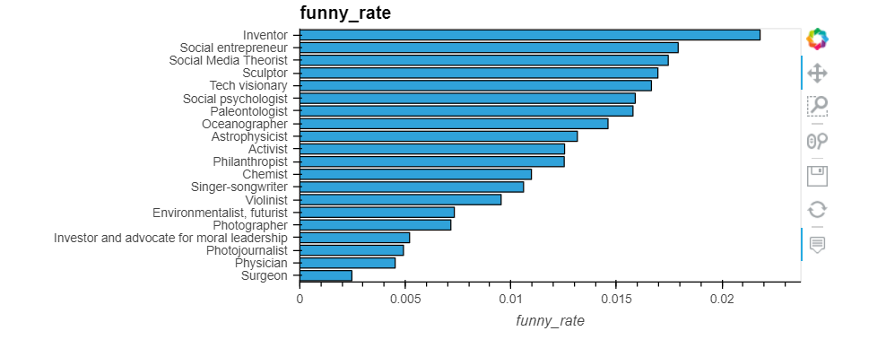
Step 3: Analyze the funny rate by occupation
speaker_occupation
Comedian                       0.512457
Actor, writer                  0.515152
Actor, comedian, playwright    0.558107
Jugglers                       0.566828
Comedian and writer            0.602085
Name: funny_rate, dtype: float64
count       2550
unique      1458
top       Writer
freq          51
Name: speaker_occupation, dtype: object
Step 4: Focus on occupations that are well-represented in the data
Writer                                51
Designer                              34
Artist                                34
Journalist                            33
Entrepreneur                          31
                                      ..
Neuroanatomist                         1
Foreign policy strategist              1
Mythologist                            1
Designer, illustrator, typographer     1
Computational geneticist               1
Name: speaker_occupation, Length: 1458, dtype: int64
pandas.core.series.Series
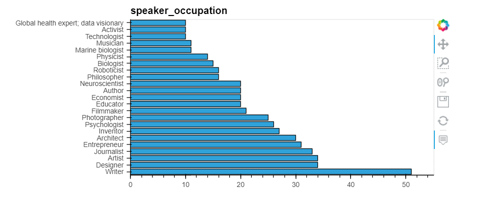
Index(['Writer', 'Designer', 'Artist', 'Journalist', 'Entrepreneur',
       'Architect', 'Inventor', 'Psychologist', 'Photographer', 'Filmmaker', 'Educator', 'Economist', 'Author', 'Neuroscientist', 'Philosopher', 'Roboticist', 'Biologist', 'Physicist', 'Marine biologist', 'Musician', 'Technologist', 'Activist', 'Global health expert; data visionary', 'Astronomer', 'Poet', 'Oceanographer', 'Graphic designer', 'Philanthropist', 'Singer/songwriter', 'Behavioral economist',
       'Historian', 'Social psychologist', 'Novelist', 'Futurist', 'Engineer',
       'Computer scientist', 'Astrophysicist', 'Mathematician', 'Comedian',
       'Photojournalist', 'Reporter', 'Evolutionary biologist',
       'Techno-illusionist', 'Writer, activist', 'Legal activist',
       'Social entrepreneur', 'Performance poet, multimedia artist',
       'Singer-songwriter', 'Climate advocate', 'Producer', 'Paleontologist',
       'Environmentalist, futurist', 'Science writer', 'Sound consultant',
       'Investor and advocate for moral leadership', 'Game designer',
       'Cartoonist', 'Tech visionary', 'Sculptor', 'Social Media Theorist',
       'Surgeon', 'Data scientist', 'Physician', 'Researcher', 'Chemist',
       'Musician, activist', 'Violinist', 'Chef'],
      dtype='object')
Step 5: Re-analyze the funny rate by occupation (for top occupations only)
(792, 24)
Lessons:
- Check your assumptions about your data
- Check whether your results are reasonable
- Take advantage of the fact that pandas operations often output a DataFrame or a Series
- Watch out for small sample sizes
- Consider the impact of missing data
- Data scientists are hilarious
Links and Resources:
- Link to data used in this tutorial: TED Talks
- Link to Full Notebook
- Part II: Comprehensive Data Analysis with Pandas — Part II
- This blog follows the talk from PyCon 2019 of Kevin Markham. PyCon: Full Conference. Kevin Markham Youtube channel: Data School
Data Analysis Project with Pandas — Step-by-Step Guide (Ted Talks Data) was originally published in Towards AI on Medium, where people are continuing the conversation by highlighting and responding to this story.
Join thousands of data leaders on the AI newsletter. Join over 80,000 subscribers and keep up to date with the latest developments in AI. From research to projects and ideas. If you are building an AI startup, an AI-related product, or a service, we invite you to consider becoming a sponsor.
Published via Towards AI
Towards AI Academy
We Build Enterprise-Grade AI. We'll Teach You to Master It Too.
15 engineers. 100,000+ students. Towards AI Academy teaches what actually survives production.
Start free — no commitment:
→ 6-Day Agentic AI Engineering Email Guide — one practical lesson per day
→ Agents Architecture Cheatsheet — 3 years of architecture decisions in 6 pages
Our courses:
→ AI Engineering Certification — 90+ lessons from project selection to deployed product. The most comprehensive practical LLM course out there.
→ Agent Engineering Course — Hands on with production agent architectures, memory, routing, and eval frameworks — built from real enterprise engagements.
→ AI for Work — Understand, evaluate, and apply AI for complex work tasks.
Note: Article content contains the views of the contributing authors and not Towards AI.
Related posts
Recent Posts


")

