Cross-Selling Web App on Streamlit Cloud

Author(s): Claudio Giorgio Giancaterino

Originally published on Towards AI.

Insurance Companies are becoming data-driven oriented with the Marketing field assuming a strategic role for the Company’s growth.

With this project, is achieved a little more knowledge of cross-selling strategy from a data science and actuarial point of view, also deploying a web app on Streamlit Cloud to share results.

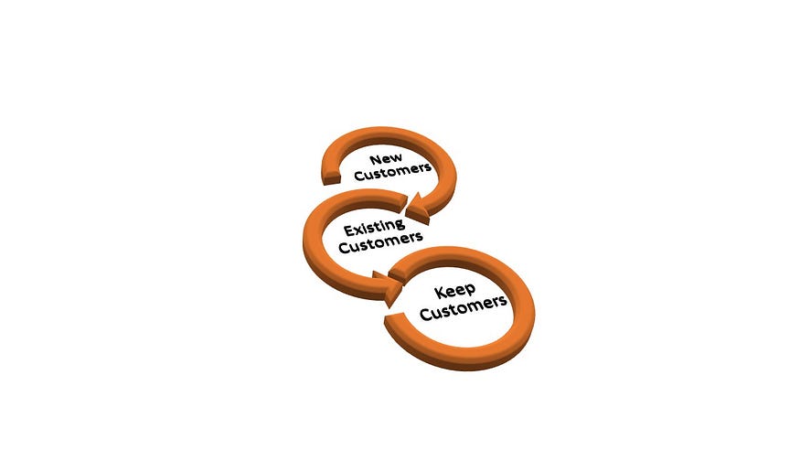
There are many ways to generate additional revenue for a Company. Introducing new products, offering additional services, or even raising prices. One common technique is known as cross-selling, which can lead to increased customer lifetime value.

In this project, using a dataset coming from a hackathon, the goal is to predict whether a customer from the past year will also be interested in vehicle insurance coverage provided by the Company.

This goal is relevant for Insurance Companies because they are becoming data-driven and customer-oriented, following other Companies' strategies from different fields. Then cross-selling modeling can lead Insurance Companies to raise revenue.

Cross-selling and up-selling are marketing terms that sound familiar, but what is the difference between each other?

Both cross-selling and up-selling are two important tools for increasing sales volume per customer. Cross-selling involves selling additional items related or complementary to a previously purchased item, while up-selling
involves increasing order volume either by selling more units of the same purchased item or upgrading to a more expensive version.

While these sales techniques are relatively old, their practice has changed with the advent of customer relationship management (CRM), and the use of information technology. I suggest reading Kamatura’s paper for more details on cross-selling.

-Exploratory Data Analysis side

I’m going ahead and looking at the dataset retrieved from the Kaggle platform: it is composed of 12 variables (including the outcome and the id) and 381.109 rows. You can follow the code from the notebook.

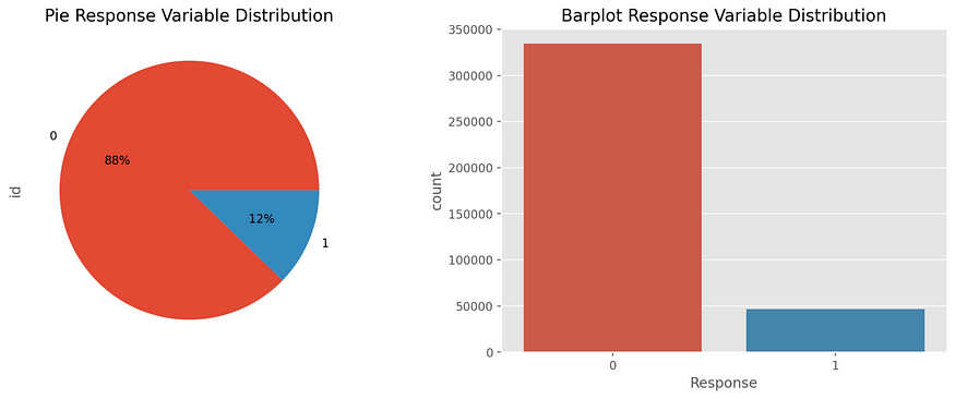
The goal of this job belongs to a classification task, and the outcome is a binary variable with class “1” for policyholders interested in purchasing the vehicle insurance, instead with class “0” for policyholders not interested in it.

def catcharts(data, col1, col2):
 plt.rcParams['figure.figsize']=(15,5)

 plt.subplot(1,2,1)
 data.groupby(col1).count()[col2].plot(kind='pie',autopct='%.0f%%').set_title("Pie {} Variable Distribution".format(col1))
 
 plt.subplot(1,2,2)
 sns.countplot(x=data[col1], data=data).set_title("Barplot {} Variable Distribution".format(col1))
 
 plt.show()

The target variable shows imbalanced classes, where only 12% of policyholders would buy the vehicle coverage.

Looking at the features, there are three numerical variables (id is dropped): Age, Annual Premium and Vintage (number of days the policyholder is in the Company portfolio).

def numcharts(data, var):
 plt.rcParams['figure.figsize']=(15,5)

 plt.subplot(1,3,1)
 x=data[var]
 plt.hist(x,color='green',edgecolor='black')
 plt.title('{} histogram'.format(var))
 plt.xticks(rotation=45)
 
 
 plt.subplot(1,3,2)
 x=data[var]
 sns.boxplot(x, color="orange")
 plt.title('{} boxplot'.format(var))
 plt.xticks(rotation=45)
 
 
 plt.subplot(1,3,3)
 res = stats.probplot(data[var], plot=plt)
 plt.title('{} Q-Q plot'.format(var))
 plt.xticks(rotation=45)
 
 
 plt.show()

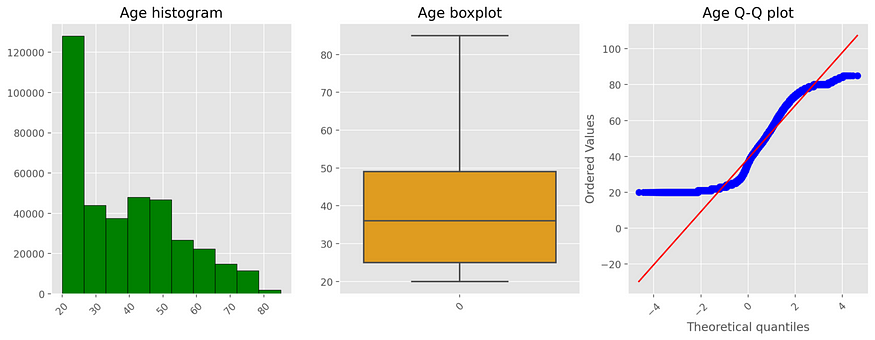
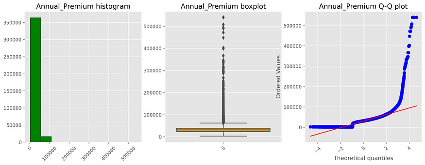
An interesting aspect to see is that owners of health coverage used for this analysis are largely young people (the median is 36). Moreover, looking at the bivariate analysis between numerical features and target variable, Age seems to be more predictive than the others, given a positive relationship with the outcome.

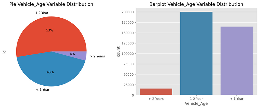
Then there are seven categorical features: Gender, Driving License, Previously Insured, Vehicle Age, Vehicle Damage, Policy Sales Channel and Region Code. The last two ones are dropped because they are not useful in the modeling activity, given that data are allocated in many classes. In the Policy Sales Channel, more or less 70% of data are covered by 3 channels; meanwhile, in the Region Code, more or less 40% of data are allocated in 2 regions and the rest in other many other not relevant region codes. Looking at the other variables, the gender variable shows a prevalence of men policyholders: 54% male vs 46% female. Almost all the policyholders have a driving license, and they own young vehicles: 53% of vehicles are in a range of 1–2 years. Most of the policyholders did not previously insure with the Company: 54% did not insure with Company vs 46% previously insured. In the last feature, vehicles with damage and without damage are equally distributed in the portfolio.

Moving toward the bivariate analysis, interesting relationships to pay attention to are coming from the relationship between Previously Insured, Vehicle Damage features and the outcome. Bivariate responses fill the class of customers not previously insured and the same bivariate response fills the class of customers with vehicle damage. The first variable can have an impact on cross-selling prediction, the second one can have an impact from the actuarial point of view as a possible risk factor in building the vehicle insurance tariff. Going ahead in the overall actuarial view, Age, Annual Premium, Gender, Vehicle Age, and Vehicle Damage are features that you can find in a typical car dataset employed to build a car insurance premium.

-Data Preparation step

Before ingesting your input features in every model, there is a pre-processing activity such as data transformation and split dataset into train and test. In the pre-processing activity, I applied the same pipeline for all models. Outliers from numerical features have been capped to avoid biased results and have been applied target encoding on categorical features instead of the classical one-hot encoding to improve the performance of models. Then have been removed predictors with zero variance because they didn’t produce any information for the models and have been removed correlated predictors to mitigate multicollinearity and improve the stability of models, though ensemble trees are less sensitive to correlated predictors. In the end, I’ve applied feature scaling to normalize the range of different input variables to a similar scale, and so to optimize the process for models sensitive to feature magnitude.

-Modelling and evaluation activity

Actually, the data preparation pursued is suitable for the Logistic Regression (LR), used as a benchmark model for this task. Logistic Regression is usually used as a reference in Insurance and also in Machine Learning comparison because it is a calibrated model, an important aspect for the evaluation of the performance.

For this job, Logistic Regression (LR) has been compared with the Gaussian Naive Bayes model (GNB), and Histogram-Based Gradient Boosting Machine (HGBM).

The choice of a Gradient Boosting algorithm comes from the fact that it is one of the best performance models, usually more competitive than Neural Networks with tabular data. Instead, the choice of Naive Bayes comes from the fact that it is another common model used in machine learning with different assumptions than Logistic Regression.

For this competition has been used the Area Under the ROC curve (AUC) is a metric for the evaluation of the performance. It assumes values between 0 and 1, with the orientation that higher values are better, but as well as the Gini index, it is not calibration—sensitive, because it ignores the marginal distribution of the outcome, leading maybe into wrong decisions. For this reason, is necessary to have a calibrated model when you look at the evaluation score. So, what is the calibration? Generally speaking, calibration is a process used to improve the reliability of a model for the estimated probabilities. A model is said well-calibrated when its predicted probabilities are close to the true probabilities of the events it is predicting. Logistic Regression is considered a calibrated model because it directly predicts the probabilities of the outcome rather than predicting the class labels based on a threshold. Each model has been evaluated in terms of calibration over the performance, and eventually, has been applied the Platt Scaling to perform a well-calibrated classifier. The Platt Scaling method transforms the outputs of a classification model into a probability distribution over classes assuming that the estimated probabilities follow a sigmoid function and fitting a logistic regression model to map the predicted probabilities to the true probabilities.

# check calibration
# Generate probability predictions from your model
def calibration(model, xdata, ydata, model_name):
 plt.rcParams['figure.figsize']=(15,5)
 probabilities = model.predict_proba(X_test)
 predicted_probabilities = probabilities[:, 1]

# Get true outcome value for each test observation
 test_outcomes = y_test

# Generate the calibration curve data
 calibration_curve_data = calibration_curve(test_outcomes, predicted_probabilities, n_bins=10)

# Plot the calibration curve
 plt.plot(calibration_curve_data[1], calibration_curve_data[0], marker='.')
 plt.plot([0, 1], [0, 1], linestyle='--')
 plt.xlabel('Predicted probability')
 plt.ylabel('Observed frequency')
 plt.title('{} Calibration Curve'.format(model_name))
 
 plt.show()

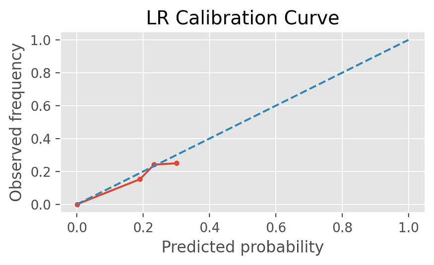
Only the Gaussian Naive Bayes has been applied to the Platt Scaling correction, and the above resulting charts show that all classifiers seem calibrated (the red predicted probability follows the blue dash true frequency of the positive label).

Looking at the results, the better model is the Histogram-Based Gradient Boosting (HGBM), which I’ve chosen as a final model to fine-tune both the hyperparameters and the threshold optimization.

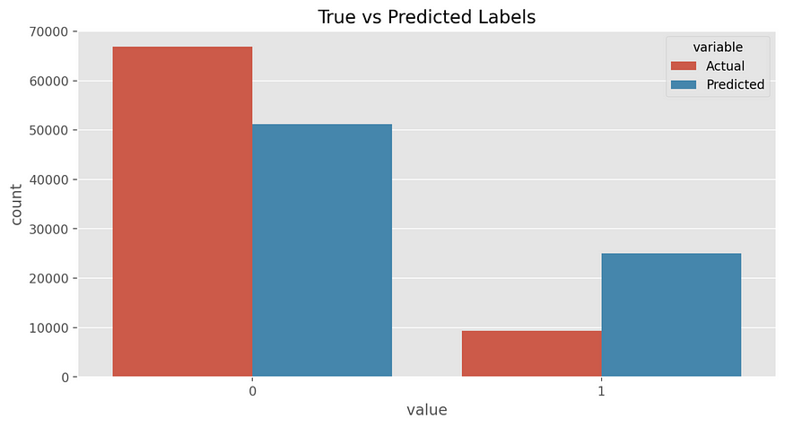
Looking at the barplot, the “0” predicted class is less underestimated, meanwhile, the “1” predicted class is overestimated.

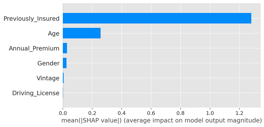
For the Feature's Importance, I’ve used the SHAP algorithm. From this algorithm, the Previously Insured feature is the most relevant in the prediction of the outcome, followed by the Age feature. This is a validation of what I’ve previously observed from the Exploratory Data Analysis. The forecast concerns if a customer is interested in a supplementary product, so the variable Previously Insured can play a relevant role in a decision. Happy customers maybe are positively oriented to buy complementary products, instead, unhappy customers prefer to leave.

Data Segmentation

Prediction is important, and it was the goal of the competition. Anyway, I’ve gone ahead looking at other aspects; with the second step, I’ve profiled customers interested in purchasing coverage using the K-Means clustering method, the more common clustering method, on numerical features and then I’ve applied this split to the overall dataset.

np.random.seed(0)
for n_cluster in range(2,10):
 clustering = KMeans(n_clusters=n_cluster, random_state=0).fit(num_sc)
 preds = clustering.predict(num_sc)
 silhouette_avg = silhouette_score(num_sc, preds)
 
 print('Silhouette Score for %i Clusters: %0.4f' % (n_cluster, silhouette_avg))

Interested Customers in buying vehicle insurance coverage can be profiled into 4 clusters resulting from the silhouette score. In this way has been possible to understand relationships between numerical features such as Annual Premium and Age with other categorical features.

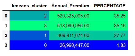
Meanwhile, the Annual Premium is distributed for 70% in the two first clusters, Age is more or less equally distributed in all clusters rather than the first one that, covers about 30% of the interested people in purchasing the vehicle coverage.

From the above charts, my attention goes toward the relationship between Annual Premium and Age vs. Previously Insured and Vehicle Damage. We can understand exactly what has been seen before, given people interested were not previously insured with the Company, so there are customers not satisfied and so not interested in purchasing complementary coverage.

Previously Insured is the most relevant feature in the prediction because, intuitively, it is linked with the satisfaction of the customers with the Company. Vehicle Damage is not relevant for the prediction, but it can have an impact on the following steps of the Company process. I mean, people interested in purchasing the complementary coverage pay an Annual Premium for vehicles with damages, and intuitively, they can have had claims, wrong driving style, and so on. Given Vehicle Damage can be a variable used in insurance coverage, this feature it’s a risk factor to consider, requiring a better analysis, because it could have an impact on the profitability of the insurance tariff.

Building the app

In the last step I’ve deployed the work realized on jupyter notebook into an app, essentially to share the results, so the inference page is not developed. Building an app with Streamlit and deploying it into the Streamlit cloud is not a hard job, though I’ve had some challenges.

I’ve built a multipage app. It requires the first “1_Cross_Selling_App.py” file as the home page and then other Python files involved in the menu, saved into the fold pages of your repository, then you can connect these files (requirements.txt included) with the cloud, and that’s it, deployment activity starts.

Visualization charts have required just little modifications of the code because the matplotlib and seaborn libraries that I’ve used for the data visualization are embedded in Streamlit.

Deployment of machine learning models has been challenging, at the first time, I repeated the same structure from the jupyter notebook, running the code, but given the small memory available in the cloud, visualization of pages requires time. The solution was to save models and run the code for the visualization of results.

In the process that followed, I started to build the app locally, then I moved into the cloud, and the hard challenge was just in this step because what worked locally, didn’t work on the cloud. It was challenging, but in the end, the solution came, and now the app is live!!!!

Final thoughts

The marketing field is growing thanks to data science activity, and also in Insurance, it is changing. The use of modern machine learning is welcome because they give a more accurate prediction (see HGBM in this job), helpful in a better allocation of costs in the marketing budget. Actuaries can play a relevant role both in the prediction and in the segmentation providing their expert judgment. Yes, because in this process, we have seen many features that are employed in the actuarial structure to develop products. Actuaries can give a risk evaluation, deep analysis of features employed in building an insurance tariff, playing as a ring conjunction between actuarial structure and marketing structure!!!
Enjoy the app U+1F60A

References

–Notebook

–App

-Dataset: Health Insurance Cross Sell Prediction U+1F3E0 U+1F3E5 U+007C Kaggle

–Cross-Selling

–Logistic Regression

–Gaussian Naive Bayes

–Histogram-Based Gradient Boosting

-Calibration

-SHAP

-K-Means clustering

Join thousands of data leaders on the AI newsletter. Join over 80,000 subscribers and keep up to date with the latest developments in AI. From research to projects and ideas. If you are building an AI startup, an AI-related product, or a service, we invite you to consider becoming a sponsor.

Published via Towards AI