Computer Vision Tutorial Series M1C2

Author(s): Sujay Kapadnis

Originally published on Towards AI.

Module 1 — Image Representation and Classification

Chapter 2— Background Replacement Of An Image

Starting here? This article is part of a computer vision Tutorial Series. Here’s where you can start.

Learning Objectives:

1. Creating a mask for an image
2. Removing the existing background of the image
3. Replacing the background with the image of our choice

Pre-Requisites: Previous Tutorials

Source: Midjourney

1. Imports

import matplotlib.pyplot as plt
import numpy as np
import cv2

2. Load the image and print the shape of the object.

image = cv2.imread('your image')
background = cv2.imread('background image')
print('Type:', type(image), 
      ' dimensions:', image.shape)

3. Function to change the colorspace

# Function to convert colorspace from BGR to RGB
def BGR2RGB(BGR_image):
    return cv2.cvtColor(BGR_image,cv2.COLOR_BGR2RGB)

image = BGR2RGB(image)
background = BGR2RGB(background)

4. Create a copy and display the image

image_copy = np.copy(image)
plt.imshow(image_copy)

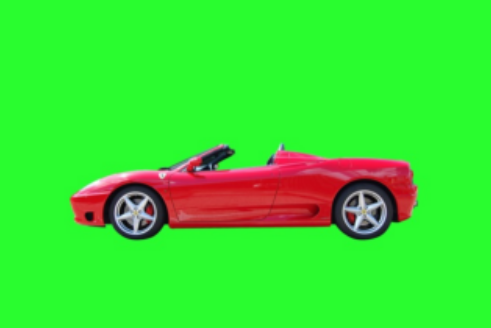Output

5. Declare Section Boundaries and create a mask

# Next step is to declare the boundaries 
lower_range = np.array([0,230,0])
upper_range = np.array([100,255,100])

# Creating a mask
masked = cv2.inRange(car,lower_range,upper_range)
plt.imshow(masked,cmap='gray')

Output

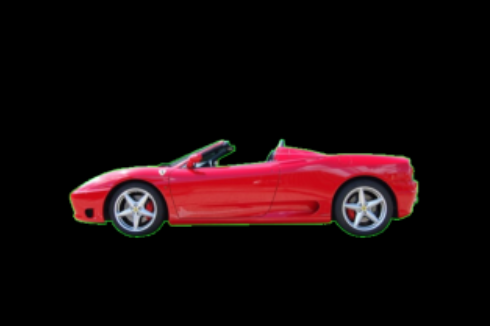
6. Using the mask on the copy of an original image

# storing original image in new variable
masked_image = np.copy(image)
# Step - 1: Region where mask value is not zero i.e not black (mask != 0) is to be turn black in newly stored original image
masked_image[mask!=0] = [0,0,0]
plt.imshow(masked_image,cmap='gray')
 

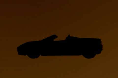
7. Using a mask on the background

# Crop the image so that it has same dimenstions as of original image
cropped_bg = background[:image.shape[0],:image.shape[1]]
# # Now Lets get to the background we need to be replace it with
# Step 2: Remove the region of car from background image
cropped_bg[mask==0] = [0,0,0]
plt.imshow(cropped_bg)

Output

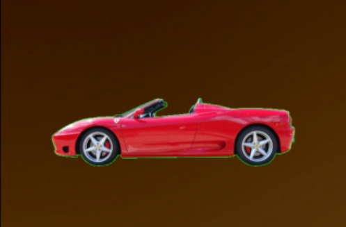
8. Final Output

As discussed in the previous tutorial, images are nothing but arrays and hence we can obtain the final output image just by adding the cropped background and masked image, like a puzzle — putting it all together.

final = cropped_bg+masked_image
plt.imshow(final)

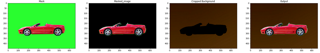
9. Plotting Function

def Plotting(mask,masked_image,cropped_bg,output_image):
    f,(ax1,ax2,ax3,ax4) = plt.subplots(1,4,figsize=(30,10))
    ax1.set_title('Mask')
    ax1.imshow(mask)
    ax2.set_title('Masked_image')
    ax2.imshow(masked_image)
    ax3.set_title('Cropped Background')
    ax3.imshow(cropped_bg)
    ax4.set_title('Output')
    ax4.imshow(output_image)

Plotting(image,masked,cropped_bg,final)

Output

10. Put it all together

# Combining Everything in one function
def BG_replacement(image,background,lower_range,upper_range):
#     Step1 - Creating a mask
    mask = cv2.inRange(image,lower_range,upper_range)
#     Step2 - Using mask on copy of original image
    masked_image = np.copy(image)
    masked_image[mask!=0] = [0,0,0]
#     Step3 - Using mask on background
    cropped_bg = background[:image.shape[0],:image.shape[1]]
    cropped_bg[mask==0] = [0,0,0]
#     Creating output image by adding images obtained in step2 and step
    output_image = masked_bulb + cropped_bg
#     Final Plot
    Plotting(mask,masked_image,cropped_bg,output_image)

Wrap Up

With this, we have completed our learning objectives for this lesson.

Declaring the section boundaries was pretty easy for this example because the background was green, and green can be easily represented by (0,255,0) in the RGB channel, but what if the background is not one of R/G/B colors? For that, I have covered one more example of a bulb with a pink-colored background. To understand how to perform the same procedure on the pink color, you can refer to this notebook.

Link to GitHub.

Upcoming:

This is it for Image Representation and Classification in the next module, i.e., Module 2: Convolutional Filters and edges we will learn:

1. Fourier Transform
2. What are filters, and how to create one
3. Gaussian kernel
4. Fourier Transform and filters
5. Canny Edge Detector
6. What is hough space and much more

This is it for this article. See you at the next one

Until then, Follow for more, and don’t forget to connect with me on LinkedIn.❤❤❤

---

Computer Vision Tutorial Series M1C2 was originally published in Towards AI on Medium, where people are continuing the conversation by highlighting and responding to this story.

Join thousands of data leaders on the AI newsletter. Join over 80,000 subscribers and keep up to date with the latest developments in AI. From research to projects and ideas. If you are building an AI startup, an AI-related product, or a service, we invite you to consider becoming a sponsor.

Published via Towards AI