Chromaticity Segmentation 🎨

Author(s): Erika Lacson

Originally published on Towards AI.

Introduction to Image Processing with Python

Episode 6: Image Segmentation — Part 2

Hello again, my fellow image-processing enthusiasts! U+1F590️ Welcome to Episode 6, the second part of our deep dive into the world of Image Segmentation! U+1F30DU+1F50D In the last episode, we explored thresholding, Otsu’s method, and the fascinating realm of color image segmentation. This time, we’re about to add more colors to our palette with Chromaticity Segmentation and the concept of Image Differencing. U+1F308

Ready for an even deeper dive into the heart of image analysis? Buckle up, because we’re taking a vibrant journey through:

• Chromaticity Segmentation U+1F3A8 (This episode)
• Image Differencing U+1F504 (This episode)

Chromaticity Segmentation U+1F3A8

When it comes to image segmentation, color plays a key role in distinguishing different regions of an image. But have you ever encountered a situation where lighting conditions made color segmentation a nightmare? U+1F4A1U+1F631 No worries, Chromaticity Segmentation is here to save your day!

Chromaticity Segmentation normalizes the RGB values of each pixel, making our segmentation independent of lighting conditions. How cool is that? We’ll dive deep into this method, exploring how we can apply it to our images to get more accurate and reliable segmentations.

But, before we start jumping in, let’s discuss the RG Chromaticity space. It’s a two-dimensional representation of the color that removes intensity values from our colors. It’s all about the proportion of the difference in color channels, mapping it in the normalized RGB space. U+1F5FA️U+1F534U+1F49A

Excited? Let’s take this journey step-by-step!

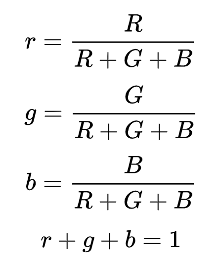
To compute the RG Chromaticity of an image, we use the following equations:

To illustrate:

This plot shows us the different colors plotted in the RG color space. Notice that we are just plotting the R and G colors, why is this the case?

Because we can compute for b just by using 1-r-g.

Let’s try segmenting our plant's image using this. But first, let’s import the necessary libraries:

# Import the necessary libraries
from skimage.io import imread, imshow
import matplotlib.colors as colors
from skimage.color import rgb2gray
import matplotlib.pyplot as plt
import numpy as np

We can use RG Chromaticity in both Parametric or Non-Parametric Segmentation.

Parametric Segmentation

The good thing about this type of segmentation combined with RG Chromaticity is that we can mask any shape.

So let’s test it out. We first need to compute the RG Chromaticity of our image:

# Display the original image
original_image = imread('plants.jpg')
plt.figure(figsize=(20,20))
plt.imshow(original_image)
plt.title('Original Image', fontsize=20, weight='bold')
plt.show()

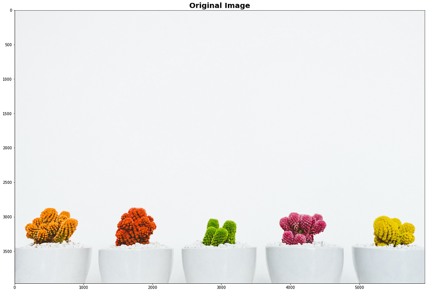
We use our equations to compute for the RG Chromaticity:

original_image_R = original_image[:,:,0]*1.0/original_image.sum(axis=2)
original_image_G = original_image[:,:,1]*1.0/original_image.sum(axis=2)

plt.figure(figsize=(20,20))
plt.scatter(original_image_R.flatten(),original_image_G.flatten())
plt.xlim(0,1)
plt.ylim(0,1);

We can compute for the 2D histogram of the color values by:

plt.figure(figsize=(20,20))
plt.hist2d(original_image_R.flatten(), 
 original_image_G.flatten(), 
 bins=100,cmap='binary')
plt.xlim(0,1)
plt.ylim(0,1);

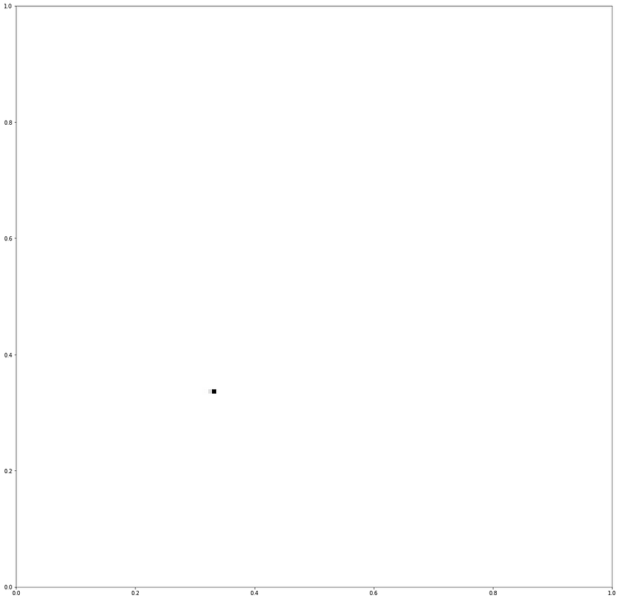
From here, we would notice what color or group of colors comprises our image. To segment our image, we would need to find a reference patch and take the RG Chromaticity of that reference image. Let’s consider the following green patch:

patch = original_image[3200:3300,2800:2900,:]
plt.figure(figsize=(10,10))
plt.imshow(patch)
plt.title('Reference Patch for Green', fontsize=20, weight='bold')
plt.axis('off');

Getting the RG Chromaticity of this patch:

patch_R = patch[:,:,0]*1.0/patch.sum(axis=2)
patch_G = patch[:,:,1]*1.0/patch.sum(axis=2)

plt.figure(figsize=(10,10))
plt.scatter(patch_R.flatten(),patch_G.flatten())
plt.xlim(0,1)
plt.ylim(0,1);

plt.figure(figsize=(10,10))
plt.hist2d(patch_R.flatten(), patch_G.flatten(), bins=100,cmap='binary')
plt.xlim(0,1)
plt.ylim(0,1);

Parametric segmentation now requires us to fit a Gaussian probability distribution using this mask. This probability distribution would dictate which pixel belongs to the color of interest. To do this, we need to compute the Mean and Standard Deviation of our object of interest.

std_patch_R = np.std(patch_R.flatten())
mean_patch_R = np.mean(patch_R.flatten())

std_patch_G = np.std(patch_G.flatten())
mean_patch_G = np.mean(patch_G.flatten())

Then, define our Gaussian Function:

def gaussian(p,mean,std):
 return np.exp(-(p-mean)**2/(2*std**2))*(1/(std*((2*np.pi)**0.5)))

Trying this out with our computed values:

x = np.linspace(0,1)
y = gaussian(x,mean_patch_R,std_patch_R)
plt.plot(x,y);

This distribution gives us the probability of color being part of our image using the R coordinate. We can actually mask our image just by using this:

prob_R = gaussian(original_image_R,mean_patch_R,std_patch_R)
plt.imshow(prob_R);

But this covers a band in our RG space. We also need to apply the G distribution.

prob_G = gaussian(original_image_G,mean_patch_G,std_patch_G)
plt.imshow(prob_G);

And since we’re considering independent probabilities, we can simply multiply the masks together:

prob=prob_R * prob_G
plt.imshow(prob)

And that’s it, we found another way to segment our image using parametric segmentation!

Non — Parametric Segmentation

For cases where our region of interest cannot be approximated by a 2D Gaussian function, we can use a non-parametric segmentation method. For this, we would use the 2D Histogram of our reference image and use histogram back-projection to mask our original image with the computed histogram of our reference patch.

plt.figure(figsize=(10,10))
plt.hist2d(patch_R.flatten(), patch_G.flatten(), bins=16,cmap='binary')
plt.xlim(0,1)
plt.ylim(0,1);

To do this, we use histogram back-projection in which we give each pixel location a value equal to it’s histogram value in chromaticity space.

Let’s test this knowledge:

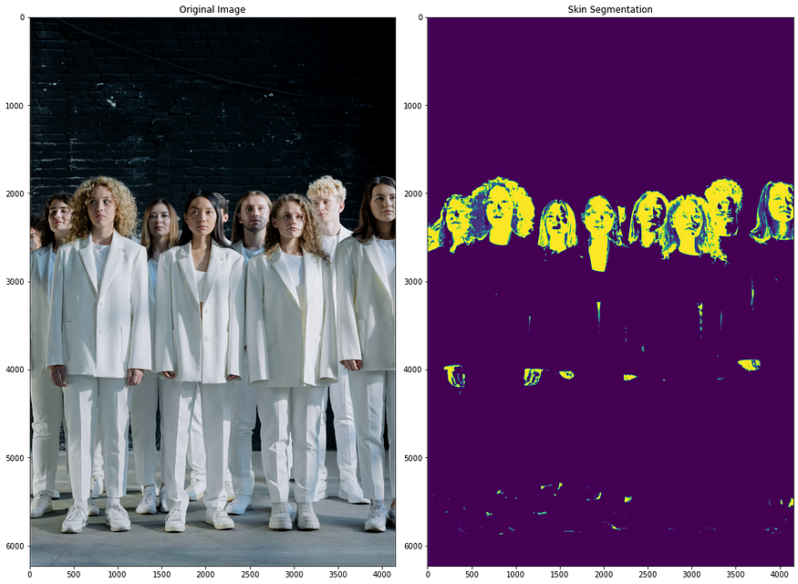
The non-parametric segmentation is especially useful for multi-color segmentation. Create a collage of different skin patch samples, then create a segmentation model by implementing the backprojection algorithm.

def backproj(patch, image):
 # Convert both images to the HSV color space
 patch_hsv = colors.rgb_to_hsv(patch)
 image_hsv = colors.rgb_to_hsv(image)

 # Compute the 2D histogram of the reference patch in the H and S channels
 patch_hist, x_edges, y_edges = np.histogram2d(
 patch_hsv[:, :, 0].flatten(), patch_hsv[:, :, 1].flatten(), bins=(6, 2) , range=[[0, 1], [0, 1]])

 # Normalize the histogram to have a maximum value of 1
 patch_hist = patch_hist / np.max(patch_hist)

 # Compute the backprojection of the image histogram using the reference patch histogram
 indices_h = np.searchsorted(x_edges, image_hsv[:, :, 0], side='left') - 1
 indices_s = np.searchsorted(y_edges, image_hsv[:, :, 1], side='left') - 1
 backproj = patch_hist[indices_h, indices_s]

 # Normalize the backprojection to have a maximum value of 1
 backproj = backproj / np.max(backproj)
 
 # Display the original image and the backprojection side by side
 plt.figure(figsize=(15, 15))
 plt.subplot(1, 2, 1)
 plt.imshow(image)
 plt.title('Original Image')
 plt.subplot(1, 2, 2)
 plt.imshow(backproj)
 plt.title('Skin Segmentation')
 plt.tight_layout()
 plt.show()

Let’s load our patch (different skin patches) and image:

patch = imread('patch.png')[:,:,:3]
plt.figure(figsize=(20,20))
plt.imshow(patch)
plt.title('Skin Patch', fontsize=20, weight='bold')
plt.axis('off');

image = imread('people.jpg')[:,:,:3]
plt.figure(figsize=(20,20))
plt.imshow(image)
plt.title('Original Image', fontsize=20, weight='bold')
plt.axis('off');

# Call the backproj function to compute the backprojection of the image
backproj(patch, image)

Well done!

Image differencing

Ever wondered how to detect changes or movements in your videos or images? Instead of segmenting by color for our regions of interest, we can instead look at the difference between two images to find our objects.

Yes, you heard it right! Image Differencing is another awesome tool that allows us to capture dynamic changes over time. U+1F550⏳

In this part of the episode, we’ll demonstrate how we successfully identified the missing item from our image using Image Differencing. It’s like playing a digital version of the classic game “Spot the Difference”! U+1F9D0U+1F50D

image1 = imread('before.png')
plt.figure(figsize=(20,20))
plt.imshow(image1)
plt.title('Original Image: Before', fontsize=20, weight='bold')
plt.axis('off');

image2 = imread('after.png')
plt.figure(figsize=(20,20))
plt.imshow(image2)
plt.title('Original Image: After', fontsize=20, weight='bold')
plt.axis('off');

Notice what’s missing? It’s easy to identify now, but what if you’re working on multiple images or videos? So that’s where Image Differencing shines. But before we do that, let’s convert the images to grayscale as it works better on grayscale images:

image1_gray = rgb2gray(image1[:,:,:3])
plt.figure(figsize=(20,20))
plt.imshow(image1_gray, cmap='gray')
plt.title('Grayscale Image: Before', fontsize=20, weight='bold')
plt.axis('off');

image2_gray = rgb2gray(image2[:,:,:3])
plt.figure(figsize=(20,20))
plt.imshow(image2_gray, cmap='gray')
plt.title('Grayscale Image: After', fontsize=20, weight='bold')
plt.axis('off');

Now, let’s perform image differencing. It’s simply a subtraction between 2 images:

diff = image1_gray - image2_gray
plt.figure(figsize=(20,20))
plt.imshow(diff, cmap='gray')
plt.title('Difference', fontsize=20, weight='bold')
plt.axis('off');

Result?

Of course, it’s the last plant. But let’s look at that in a colored version:

diff = image1_gray - image2_gray
plt.figure(figsize=(20,20))
imshow(diff)
plt.title('Difference', fontsize=20, weight='bold')
plt.axis('off');

There you have it, the missing piece. Not a perfect color conversion, though. But the important part is we were able to use it to find what was missing.

Conclusion U+1F3C1

Wow! What an exciting journey it’s been! We ventured deeper into the vibrant realm of Chromaticity Segmentation, learning to normalize our RGB values and accurately segment our people images with different skin colors. U+1F308U+1F4A1

We also explored the dynamic world of Image Differencing, learning to capture changes over time and detect movements in our videos or images. U+1F504U+1F39E️

As we wrap up this episode, remember, my fellow image-processing enthusiasts, these techniques are just tools in your toolbox. It’s a problem you’re trying to solve, and the creativity you bring that really makes the magic happen! U+1F9D9‍U+2642️U+2728

Stay curious, keep learning, and never stop exploring the world of pixels. Because every pixel has a tale to tell, and you, my friend, are the storyteller. U+1F3A8U+1F4D6

Until next time, keep coding, keep exploring, and most importantly, have fun! See you in the next episode! U+1F680U+1F469‍U+1F4BBU+1F468‍U+1F4BBU+1F31F

References:

• Borja, B. (2023). Lecture 6: Image Segmentation Part 2 [Jupyter Notebook]. Introduction to Image Processing 2023, Asian Institute of Management.

Join thousands of data leaders on the AI newsletter. Join over 80,000 subscribers and keep up to date with the latest developments in AI. From research to projects and ideas. If you are building an AI startup, an AI-related product, or a service, we invite you to consider becoming a sponsor.

Published via Towards AI