


 — Using Python")
Capital Assets Pricing Model (CAPM) — Using Python
Last Updated on May 24, 2022 by Editorial Team
Author(s): Jayashree domala
Data Visualization, Programming
Capital Assets Pricing Model (CAPM) — Using Python
A guide to knowing about CAPM and implementing it in Python.
What is CAPM?
The capital asset pricing model (CAPM) is very widely used and is considered to be a very fundamental concept in investing. It determines the link between the risk and expected return of assets, in particular stocks.
What is the CAPM equation?
The CAPM is defined by the following formula:
where ‘i’ is an individual stock
r(i)(t) = return of stock ‘i’ at time ‘t’
β(i) = beta of ‘i’
r(m)(t) = return of market ‘m’ at time ‘t’
α(i)(t) = alpha of ‘i’ at time ‘t’
β of a stock ‘i’ tells us about the risk the stock will add to the portfolio in comparison to the market. β=1 means that the stock is in line with the market.
According to CAPM, the value of α is expected to be zero and that it is very random and cannot be predicted.
The equation seen above is in the form of y = mx+b and therefore it can be treated as a form of linear regression.
How to implement it in Python?
→ Install packages
The scipy package will be used. It has a function to calculate the linear regression. Along with it, pandas is imported to deal with data and the data is obtained using pandas datareader. Visualizations are done through matplotlib.
>>> from scipy import stats
>>> import pandas as pd
>>> import pandas_datareader as web
>>> import datetime
>>> import matplotlib.pyplot as plt
>>> %matplotlib inline
→ Data
The start and end dates are defined and the analysis is done in this interval itself.
>>> start = datetime.datetime(2013,1,1)
>>> end = datetime.datetime(2016,1,1)
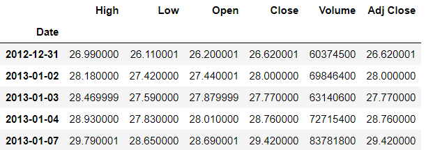
Get the data for a market such as ‘SPY’ (SPDR S&P 500).
>>> df_spy = web.DataReader('SPY','yahoo',start,end)
>>> df_spy.head()
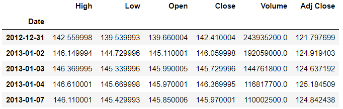
Next, the data for a stock is obtained. The stock used here is Facebook.
>>> df_fb = web.DataReader('FB','yahoo',start,end)
>>> df_fb.head()
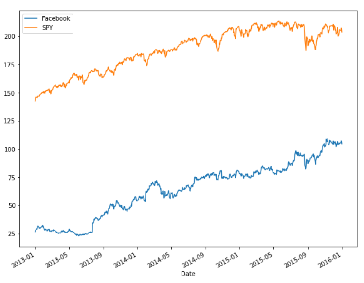
→ Visualize
According to CAPM, there should be some relation between the stock performance and market performance which will be looked into ahead.
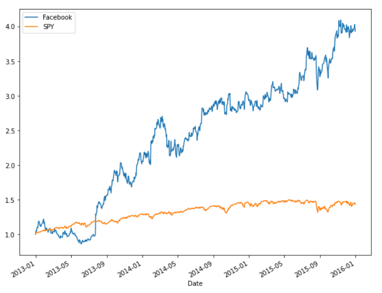
>>> df_fb['Close'].plot(label = 'Facebook', figsize=(10,8))
>>> df_spy['Close'].plot(label = 'SPY')
>>> plt.legend()
→ Statistics
As seen from the plot, it seems like the stock performance is mimicking the market performance. So statistically they can be compared. The cumulative returns are found.
>>> df_fb['Cumu'] = df_fb['Close']/df_fb['Close'].iloc[0]
>>> df_spy['Cumu'] = df_spy['Close']/df_spy['Close'].iloc[0]
>>> df_fb['Cumu'].plot(label = 'Facebook', figsize=(10,8))
>>> df_spy['Cumu'].plot(label = 'SPY')
>>> plt.legend()
The daily return is also determined.
>>> df_fb['daily_ret'] = df_fb['Close'].pct_change(1)
>>> df_spy['daily_ret'] = df_spy['Close'].pct_change(1)
>>> plt.scatter(df_fb['daily_ret'],df_spy['daily_ret'])
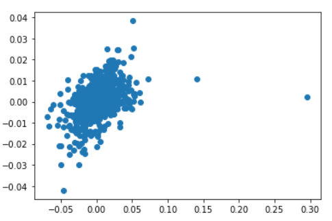
The scatter plot indicates that there is some relation between the daily returns of the stock and the market.
→ Finding alpha and beta values
The alpha and beta values are found by using the stats package of scipy and calling the linear regression function of it. While finding the daily returns, the first row has NaN values and therefore while passing the columns for linear regression everything from the first row is considered.
>>> LR = stats.linregress(df_fb['daily_ret'].iloc[1:],df_spy['daily_ret'].iloc[1:])
>>> LR
LinregressResult(slope=0.14508921572501682, intercept=0.0002066678439426573, rvalue=0.41761756846081083, pvalue=2.8903149350900316e-33, stderr=0.011496201726453189)
The linear regression model is built. It has 5 values which can be obtained through tuple unpacking. The five values are beta, alpha, rvalue, pvalue and standard error.
>>> beta,alpha,r_val,p_val,std_err = LR
>>> beta
0.14508921572501682
>>> alpha
0.0002066678439426573
Take a note that as the CAPM said that alpha is close to zero, it can be seen here too. And the beta value is high if the stock behaves just like the market. Therefore the beta value is really low here as there is not much relation between them.
Refer to the notebook here.
Reach out to me: LinkedIn
Check out my other work: GitHub
Capital Assets Pricing Model (CAPM) — Using Python was originally published in Towards AI on Medium, where people are continuing the conversation by highlighting and responding to this story.
Published via Towards AI
Towards AI Academy
We Build Enterprise-Grade AI. We'll Teach You to Master It Too.
15 engineers. 100,000+ students. Towards AI Academy teaches what actually survives production.
Start free — no commitment:
→ 6-Day Agentic AI Engineering Email Guide — one practical lesson per day
→ Agents Architecture Cheatsheet — 3 years of architecture decisions in 6 pages
Our courses:
→ AI Engineering Certification — 90+ lessons from project selection to deployed product. The most comprehensive practical LLM course out there.
→ Agent Engineering Course — Hands on with production agent architectures, memory, routing, and eval frameworks — built from real enterprise engagements.
→ AI for Work — Understand, evaluate, and apply AI for complex work tasks.
Note: Article content contains the views of the contributing authors and not Towards AI.
Related posts
Recent Posts

")


Comments are closed.