
A Quick Introduction to Machine Learning: Part-2 (Regression)
Last Updated on July 17, 2023 by Editorial Team
Author(s): Abhijith S Babu
Originally published on Towards AI.
In this article, we are going to see some of the supervised learning techniques. Before reading this article, read part-1 to have a basic idea about supervised learning.

One of the commonly used methods in supervised learning method is regression. Regression is a method that is used to find a mathematical relationship between different variables in data. To understand regression, let’s take the land pricing example. The price of a plot is found to be dependent upon various factors such as climate, location, nearby facilities, and so on. All of these can be numerically quantified. From all these input variables, we have to find a mathematical function that outputs the target variable, that is, the price of land. Let us have a look at the most basic regression method — simple linear regression.
Simple Linear Regression
Simple linear regression is used to find a linear relationship between two variables. Consider the land pricing problem where the price of land is having a linear relationship with the distance from the city center. Let us take a small hypothetical example for that.

Let us plot this data on a graph and see.
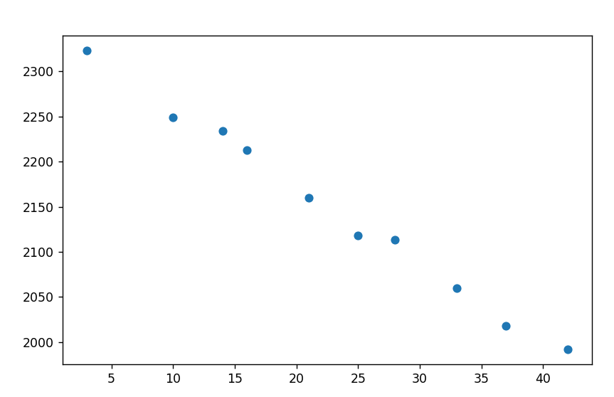
Here we can see that the plot almost forms a straight line…
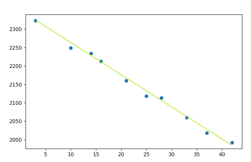
So the relationship between the two variables has to be similar to the equation of a straight line : y = mx + c
In this case, x is the distance and y is the price. m is the slope of the line and c is the y-intercept. Our job is to find m and c. Here I am going to explain two methods to find m and c
Ordinary least square method.
We have to find m and c such that the line gives the best solution to our problem. The best solution is one in which the difference between the value predicted, and the actual value is least. Look at the given figure.

Here the line is not a better solution than the previous one because, in many of the cases, the predicted value is far from the actual value. Let the actual value be t, and the predicted value be p. We have to minimize the difference between p and t for all the points in the dataset. For that, we can take the sum of squared difference, i.e. take the square of (p-t) and sum it for all the points in the data. We have to minimize the sum of squared differences by choosing the appropriate value of m. Thus, we apply some calculus and we found an equation for m
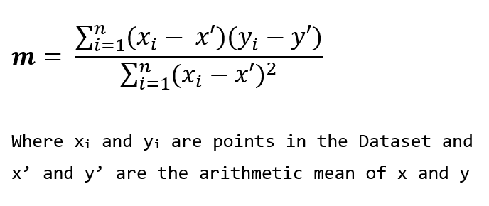
From the value of m, we can find the value of c using the formula
c = y’ — mx’
where y’ and x’ are the arithmetic means of y and x. Using these formulas, you can find the line that best fits a given set of data.
Gradient descent
Another method for finding the best-fit line is gradient descent. Here we use a bit of differential calculus to approximate the actual value of m and c in the equation. For better understanding, first let us assume a random value for c, say 0. Now we are going to find the best possible value of m, given c is zero. The sum of squared error denotes the error between the actual value and the predicted value. We can see that the error and slope(m) have a quadratic relationship. If we vary the value of m and find the error for each value, we will get a plot like this.
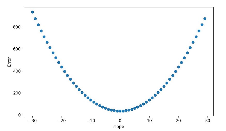
Since our aim is to minimize the error, we have to find the slope corresponding to the lowest point in the above plot, which is a minima. First, we assume a random value for m, let it be -25 in this case. Now, we have to move it towards the minima. In a quadratic curve with a minima, we know that the derivative of a point (slope of the curve at a point) is negative infinity at the left end and it increases and becomes zero at minima and goes on to increase as we move right. So we have to subtract our m with a term containing the derivative of the curve to reach minima quickly. By doing this for several iterations using our input dataset, we can find the value of m, close to minima. Here, note that the exact value of minima cannot be found.
(Note that we talk about 2 slopes here, one is the slope m of the best fit line and the other is the slope of the quadratic curve. Don’t get confused between the two slopes)
The value of c also has a quadratic relationship with the error function in a similar manner. Now that we have got the value of m, we can find the value of c, in the same way, using the value of m we got. The gradient descent method combines these two steps. We assume a random value for m and c in the beginning. Then by calculating the derivative, we can vary the value of m and c simultaneously in each iteration. If we continue for a large number of iterations, we can reach an optimal value of m and c. Thus we can find the best-fit line.
Multiple Linear Regression
So far, we have seen two methods to do simple linear regression. Now look at the land pricing problem. So far, we took the distance from the city center as the input variable. But we know that there are other factors that affect the price of land, say the distance from the nearest supermarket. Now we have to include that as a variable as well. Here we know that more than one variable has a linear relationship with the target value. This can be solved using multiple linear regression.
If there are multiple variables involved, the equation that shows their relationship looks like this.

Similar to simple linear regression, our goal is to find the values of all the coefficients of x and c, such that the sum of the difference between the predicted value and actual value is the least. The procedure for finding the coefficients is very complicated. There are various packages available in Python programming language that can be used to perform these functions.
Another case of regression is polynomial regression, in which the relationship between the variables might be non-linear. It can be quadratic, cubic, and so on. Here also, the relationship equation might contain a large number of coefficients and the math to find them is much more complicated. Packages in the Python programming language can be used to solve these problems. Now let us have a look at logistic regression.
Logistic regression
So far, we have seen cases where we predict some continuous values. For example, the price of land can be 1850, 2684, 2139.86, and so on. But what if it is a classification problem. Suppose you want to classify the images of cats and rabbits. The target variable can only take two values — cat or rabbit. Let us quantify it by assigning 0 to cats and 1 to rabbits. Our target variable should only take the value 0 or 1. If we use the previous regression methods, we might get -17.26, 0.67, or 53 as the output. So we need a function that approximates the output to one of the two values.
Extracting features from images is complicated in this scope, so I will take a simple example. You want to predict if it will rain tomorrow or not based on today’s temperature. Our input variable is temperature, which can take values between 10 and 45. The output variable takes the value 0 if it doesn’t rain and 1 if it rains.
Take the following hypothetical graph.

Here we can see that when the temperature is higher, it is more likely to rain. We need a curve that fits maximum number of points in this plot, but also never goes below 0 and never goes above 1. A curve like this will help.
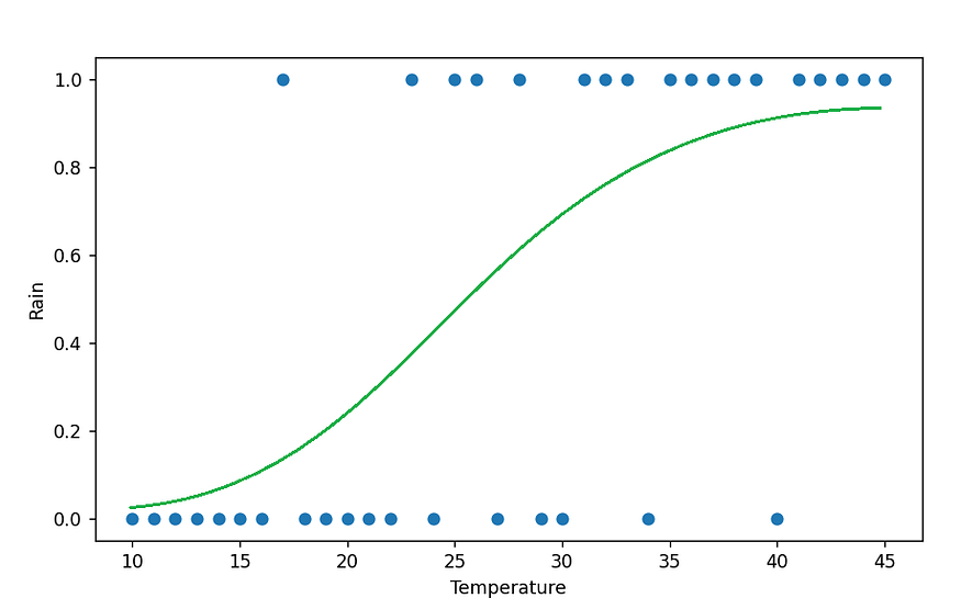
This curve runs between 0 and 1. It can be used to denote the probability that we get 1 as the output for a particular input. So in the above example, when the temperature is close to 45, the probability of rain is very close to 1, while a temperature close to 10 will give the probability of rain close to zero. We have a function that does the trick. It is called a logistic function. It gives a similar curve which reaches 1 at infinity and 0 at negative infinity. The standard logistic equation is
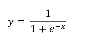
We can modify x in the equation based on our data to create a curve that can help us make predictions. Instead of x, we give a linear function of x, that is mx + c. So the probability of getting 1 as the output can be given by
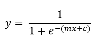
Now that we have the predicted y(probability of getting 1) and the actual value(0 or 1), we can use the gradient descent method discussed above to find the best value of m and c.
In this article, we have seen various types of regression that can be used in supervised learning. In part-3, we will see other important machine learning techniques. Follow me to get the upcoming parts. Give your doubts and suggestions in the response and they will be considered in the upcoming parts. Happy reading!!!
Join thousands of data leaders on the AI newsletter. Join over 80,000 subscribers and keep up to date with the latest developments in AI. From research to projects and ideas. If you are building an AI startup, an AI-related product, or a service, we invite you to consider becoming a sponsor.
Published via Towards AI
Towards AI Academy
We Build Enterprise-Grade AI. We'll Teach You to Master It Too.
15 engineers. 100,000+ students. Towards AI Academy teaches what actually survives production.
Start free — no commitment:
→ 6-Day Agentic AI Engineering Email Guide — one practical lesson per day
→ Agents Architecture Cheatsheet — 3 years of architecture decisions in 6 pages
Our courses:
→ AI Engineering Certification — 90+ lessons from project selection to deployed product. The most comprehensive practical LLM course out there.
→ Agent Engineering Course — Hands on with production agent architectures, memory, routing, and eval frameworks — built from real enterprise engagements.
→ AI for Work — Understand, evaluate, and apply AI for complex work tasks.
Note: Article content contains the views of the contributing authors and not Towards AI.


