A guide to Predictive Lead Scoring using Machine Learning

Author(s): Yashashri Shiral

Originally published on Towards AI the World’s Leading AI and Technology News and Media Company. If you are building an AI-related product or service, we invite you to consider becoming an AI sponsor. At Towards AI, we help scale AI and technology startups. Let us help you unleash your technology to the masses.

A Guide To Predictive Lead Scoring Using Machine Learning

Lead scoring is a valuable tool while implementing a marketing strategy, and in this article, you will understand how you can do it using Machine learning.

In the article, I’m covering →

1. What is lead scoring, and why it’s important
2. Types of lead scoring
3. Understanding Data
4. Exploratory Data Analysis & Observations
5. One Hot Encoding
6. Feature Selection — RFE
7. Variance Inflation Factor
8. SMOTE — oversampling
9. Model Implementation — Logistic Regression, Hyperparameter Tuning
10. Model Evaluation

Refer to my GitHub repo here -> https://github.com/YashashriShiral/LeadScoring

1. What is lead scoring, and why it’s important?

The purpose of marketing is to reach your target audience and communicate the benefits of your product and get people interested in the products and services. So you can successfully acquire, keep and grow. However, the more leads you generate, the more selective you have to be in your pursuits. Sales representatives don’t want to waste time chasing a large list of leads. Since sales operation has high cost both in time and money, they should focus on nurturing only the most engaged and fitted leads in order to improve and maintain a profitable ‘Return of Investment.’ To consistently find strong potential customers, sales reps need a lead scoring model. In short, lead scoring is the process of qualifying prospects so salespeople can do their job more efficiently. Focus on lead generation would drive traffic from high-quality prospects(potential clients, someone who is in the market for your product has resources needed to buy it but has not purchased it). And high-quality prospects come with high-value customers that mean more revenue for your business. In other words, the idea is to assign scores to all prospects based on how their characteristics match with the pre-established profile of converted customers. The leads that score above a specific threshold are considered an ideal target.

Even though the companies recognize the importance of sales and marketing alignment, some still struggle with it. The sales team complains about marketing is spending money on campaigns that are not generating value, and marketing complains that the leads they are delivering aren’t getting converted. So Lead Scoring gives your marketing and sales team a common valuation system they can use to determine which of those leads to follow up.

Using lead scoring, you can achieve the following:

1. Increase Sales Efficiency
2. Increase Marketing Effectiveness
3. Improve sales and Marketing Alignment
4. Increase Revenue
5. Streamline your time and impact

2. Types of Lead Scoring:

1. Rules-based lead scoring-

You take a look at common patterns and attributes among the customers that converted for your business and create a score based on interaction with Sales/Marketing teams. In this, whatever actions that customers are taking you are assigning values to them based on how important those actions are to the business.

e.g. 5(points) Page view + 10(points) downloading content + 15(points) Attending webinar + 3(points) click on links .
As a user completes these actions, you can add up the point values for each of these actions and determine how likely someone is to be a good fit for your product. You can certainly use python and SQL to automate this process. Some companies rely on this method because they like the personal aspect of lead scoring. No one knows your customer better than one who spends time convincing them to become customers (sales)

2. Predictive Lead Scoring-

Predictive lead scoring is an algorithm-based machine learning approach to lead scoring. In this method, the algorithm learns patterns based on your customer purchases and behavioral data to predict what is the possibility that the customer will make a purchase. Predictive scoring identifies hidden buying signals that would have been impossible to find manually. In this article, we are taking a predictive lead scoring approach.

3. Input Data:

I’m using a dataset from the UCI Machine learning repository. You can download it from here.

Dataset information: The data is related to direct marketing campaigns of a Portuguese banking institution. The marketing campaigns were based on phone calls. Often, more than one contact with the same client was required in order to access if the product (bank term deposit) would be (‘yes’) or not (‘no’) subscribed.

So in the dataset, we have customers’ personal information, their contact activity information, previous campaign information, and some social stats, and we also have information about which leads are converted and not converted yet. Our job is to help select the most promising leads. Build a model wherein you need to assign a lead score to each of the leads such that customers with higher scores have higher conversion chances and customers with lower lead scores have lower conversion chances.

I’m building a logistic regression model to assign a lead score between 0 and 100 to each of the leads, which can be used by the company to target potential leads. A higher score would mean that the lead is hot, i.e. is most likely to convert, whereas a lower score would mean that the lead is cold and will mostly not get converted.

Attribute Information:

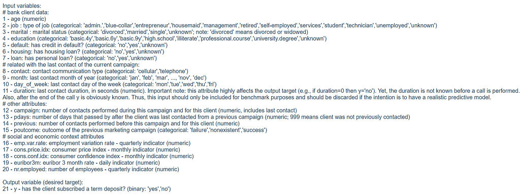
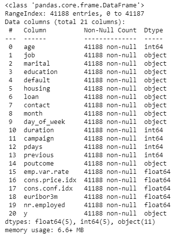
You have three types of attributes in the data:

I’m dropping the ‘duration’ attribute — based on attribute information Important note: this attribute highly affects the output target (e.g., if duration=0, then y=’no’). Yet, the duration is not known before a call is performed. Also, after the end of the call, y is obviously known. Thus, this input should only be included for benchmark purposes and should be discarded if the intention is to have a realistic predictive model.

Customer information: age, job, marital, education, default, housing, loan

Contact activity information: contact, month, day_of_week

Campaign activity information: campaign, pdays, previous, poutcome

Social and economic context: emp.var.rate, cons.price.idx, cons.conf.idx, euribor3m, nr.employed

4. Exploratory Data Analysis:

Based on analysis: Customer age range from 17–98, and 40% of the customers are in the range between 30–40. And younger and older customers tend to convert more than middle-aged ones.

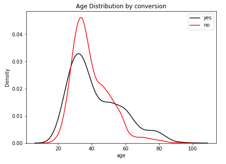
You can start plotting graphs to understand the distribution of variables.

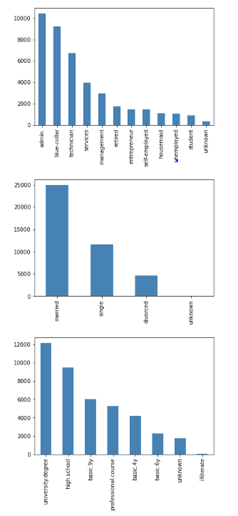
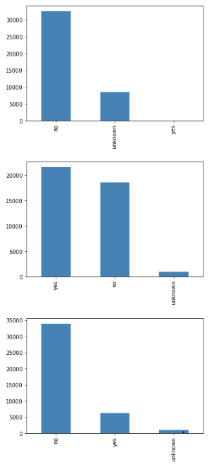
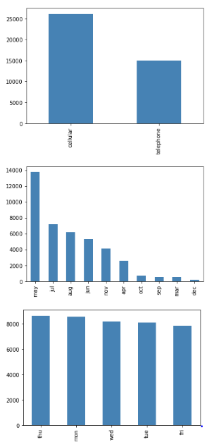
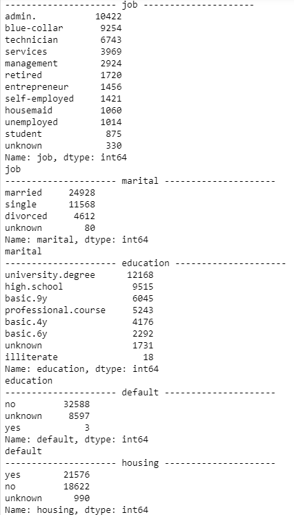
You can plot all the variables or print the distribution like above.

Now what I’m doing here is mapping the distribution of converted/not converted (yes/no) target feature(y) with respect to all the variables we have. To understand which features are important for analysis and what the distribution looks like for them.

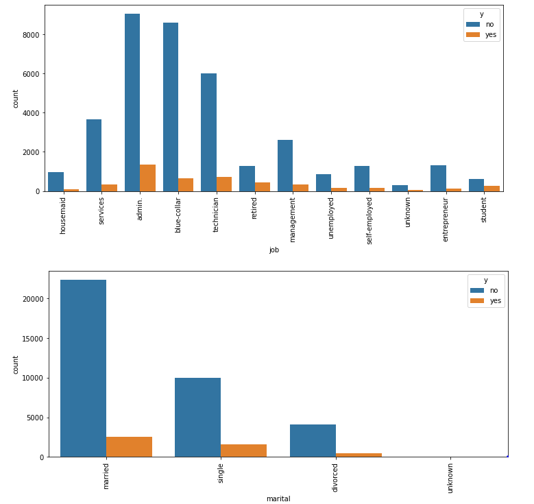
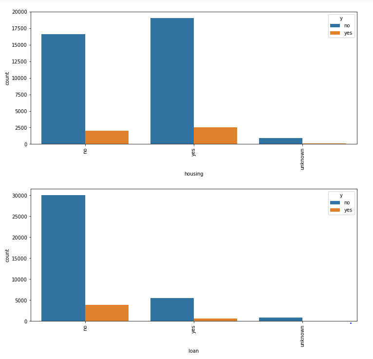
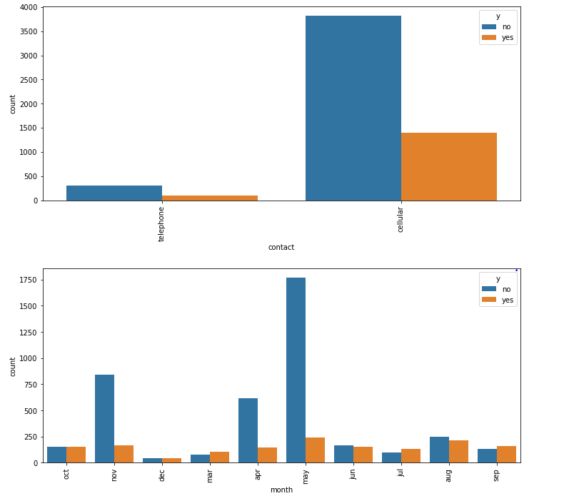
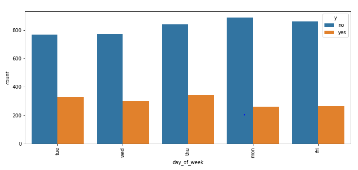
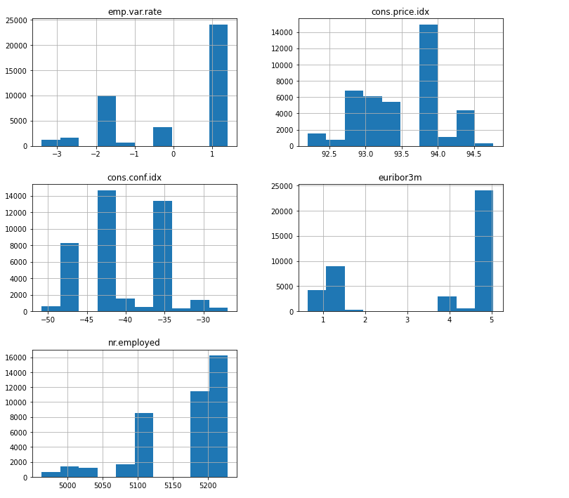
Observations based on the graphs above:

• Younger and Older customers are most likely to get converted in comparison with middle age
• Retired/students are most likely to get converted
• Singles have high chances of conversion
• If a customer who has a high school education will get converted
• If a customer has no credit in default, have a greater chance of getting converted
• If a customer who has cellular contact has more chance of getting converted
• If contacted in the Month of March/Sep/Dec, there is a better chance of the customer getting converted
• If called on Weekday Tue/Wed/Thru will have a better chance of customer getting converted
• If there is no previous loan good chance of the customer getting converted

Please bear with me as we are halfway through our project here. The difficult part of understanding what’s in the data is almost done.

Now we just have to use the proper statistical tools and do predictions. Let’s start with the understanding of the correlation between variables(an important method for feature selection)

Pearson Correlation:

Correlation is a way of finding how well the variables are related. Pearson correlation shows the linear relationship between the data.

• 1 indicates a strong positive relationship
• -1 indicates a strong negative relationship
• 0 indicates no relationship at all

Now let’s see what correlation looks like for the economic context numerical variables that we have.

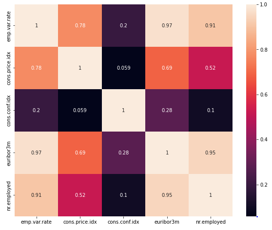
You can see that there is a high correlation of ‘cons.price.idx’ with other economic numeric variables and a high correlation between nr.employed and emp.var.rate , euribor3m. This means multicollinearity exists in our data.

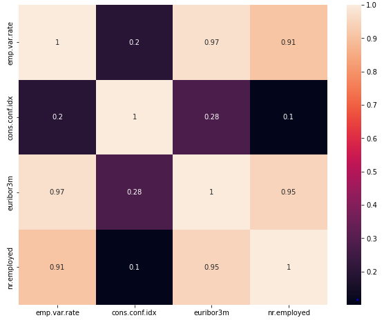
correlation for all numerical variables

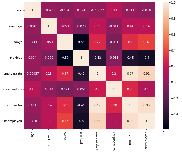
You have a weak correlation between the above numerical features.

5. One Hot Encoding:

Now, as we know, we have a lot of categorical variables in the data, which we need to convert into numerical form if we want to run any ML Model on the data. Please refer to my previous article if you want a detailed understanding of Encoding — here.

In one hot encoding for each categorical variable, it creates a new numerical variable.

I wanted to see the correlation between variables after encoding

I know there is a lot happening in this graph let’s break it down:

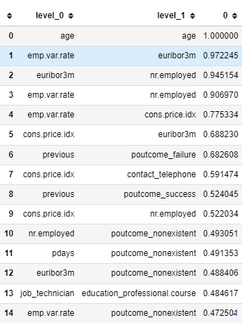
As we observed before that there is a positively strong correlation between socio-economic variables, but there is no strong correlation between other variables. There is little less than a strong correlation between ‘previous’ and ‘poutcome_failture’. Let’s keep this in mind for now.

There is a negative correlation between ‘default_no’ , ‘default_unknown’ & ‘housing_yes’ , ‘housing_no’ & ‘pdays’, ‘poutcome_success’ & ‘loan_yes’, ‘loan_no’. This means you have multicollinearity in variables. (it occurs when independent variables in regression problem are highly correlated)

Now we will select important features and try and reduce multicollinearity between variables.

6. Feature Selection:

Recursive Feature Elimination (Wrapper Method)

Feature selection is a way of reducing the input variables for the model by only using relevant data in order to reduce the overfitting model. Feature selection helps in the signification of the model so that it can be easily interpreted.

Wrapper Method: In the wrapper method, feature selection is based on a specific machine learning algorithm that we are trying to fit on a given dataset. It follows a greedy search approach by evaluating all the possible combinations of features against the evaluation criterion.

Recursive Feature Elimination: The goal of RFE is to select features by recursively considering smaller and smaller sets of features. First, the estimator is trained on the initial set of features, and the importance of each feature is obtained. Then, the least important features are pruned from the current set of features. That process is recursively repeated on the pruned set until the desired number of features to select is eventually reached.

These are the 15 important features we are getting after using RFE.

Now let’s see if these variables still persist in any multicollinearity or not using Variance inflation Factor.

7. Variance Inflation Factor: Multicollinearity

When some features are highly correlated, we might have difficulty distinguishing between their individual effects on the target variable. VIF is used to detect multicollinearity between variables. VIF is calculated as (1/1-R-squared) where R-squared is determined in linear regression, and its value lies between 0 & 1. So, the greater the R-Squared greater the correlation and the greater VIF. Generally, VIF above 5 indicated high multicollinearity.

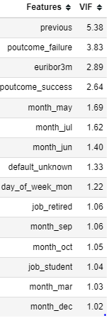
As you can see ‘previous’ feature has a VIF value that is more than 5. Let’s eliminate that feature from the final list.

The final list of features → [ ‘euribor3m’, ‘job_retired’, ‘job_student’,
‘default_unknown’, ‘month_dec’, ‘month_jul’, ‘month_jun’, ‘month_mar’,
‘month_may’, ‘month_oct’, ‘month_sep’, ‘day_of_week_mon’,
‘poutcome_failure’, ‘poutcome_success’]

Almost there, now as we have important features, let’s move on to the model implementation.

Before we move on to model implementation, there is one more step that we will have to do is — oversampling data.

8. SMOTE Oversampling

As you can see, we have fewer customers who got converted(yes/1), i.e. 3,252

So basically, the dataset that we are using is imbalanced. The reason we can’t ignore this imbalance dataset is it would give a poor performance on the minority class, which is when a customer got converted(yes/1).

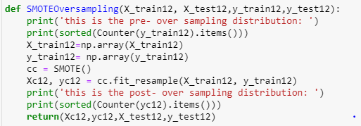
One of the ways of approaching an imbalanced dataset is to do the over-sampling of the minority class. SMOTE(Synthetic Minority Over-sampling Technique) is one such technique that synthesizes new examples from minority classes by selecting examples that are close in the feature space.

Great success!!! Now let’s implement Logistic Regression.

Model Implementation: Logistic Regression

What is Logistic Regression: Logistic Regression is a predictive analysis used for solving binary classification problems. Logistic regression estimates the probability of an event occurring, such as voting or didn’t vote, based on a given dataset of the independent variables. Since the outcome is a probability, the dependent variable is bounded between 0 and 1.

For a detailed understanding of logistic regression, refer to these articles →

1. https://learn.g2.com/logistic-regression
2. https://towardsdatascience.com/logistic-regression-detailed-overview-46c4da4303bc

We are using logistic regression because, as mentioned above, it’s used in predicting categorical variables such as if the email is spam or not.(yes/no)

I’m using both scikit-learn and statsmodels libraries. Both libraries work a little differently for logistic regression. I’ll explain how →

scikit-learn → If the model fails to generalize the data, we run into overfitting the training data. By default, scikit-learn, lib applies regularization. Regularization balances the need for predictive accuracy on the training data. Increasing penalty reduces the coefficients and hence reduces the likelihood of overfitting. If the penalty is too large, it will reduce predictive power on both the train and test datasets. We can use GridSearchCV to choose optimal parameters for the model.

Hyperparameter Tuning:

Hyperparameters are internal coefficients or weights for a model found by the learning algorithm. Unlike parameters, hyperparameters are specified by the developer when configuring the model. In this scenario, the challenge is to know what values to use for the hyperparameters of a given algorithm on a given dataset, therefore, we use GridSearchCV.

Now we will use these hyperparameters in our logistic regression model.

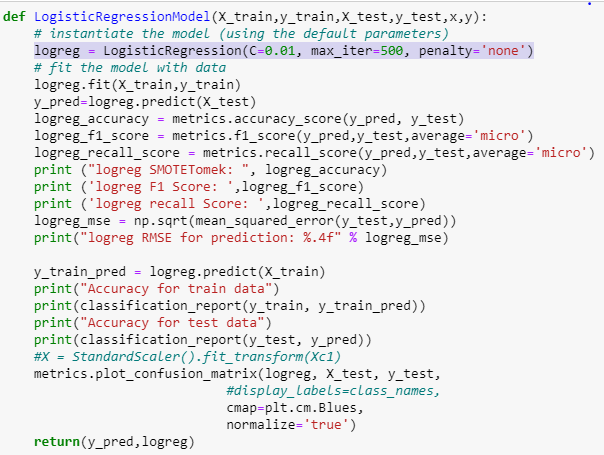
Let’s first quickly understand model evaluation →

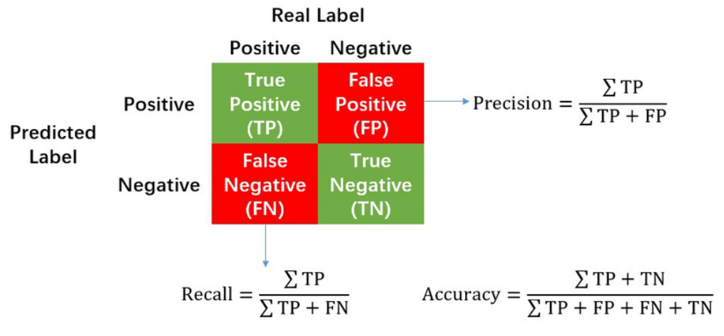
The confusion matrix shows the number of correct/incorrect predictions made by the classification model compared to the actual outcomes in the data.

Accuracy: How often model is correct

Precision(positive predictive value): The proportion of positive cases that were correctly identified. What percentage is truly positive?

Recall(Sensitivity): The proportion of actual positive cases which are correctly identified. What percentage are predicted positive?

ROC AUC Curve: When we want to visualize or check the performance of the classification model, we use AUC(Area under the curve) and ROC(Receiver Operating Characteristic). ROC is a probability curve, and AUC represents the degree or measure of separability. The higher the AUC better the model is predicting actual values.

Scikit-learn Model output:-

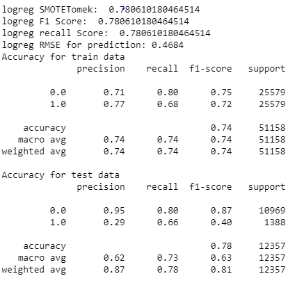
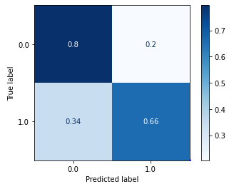
We can see that accuracy of train data is 74% and test data is 78% which indicates that we are not overfitting the data and we have good value for recall i.e. means, 66% of the time, we are correctly predicting that the customer is converted.

Out of 1388 converted customers in the test dataset model is able to predict 914 correctly.

Statsmodels Understanding:

As I mentioned before, I’m also using statsmodels, in this library, regularization is turned off by default. Another point to remember is stats model does not include intercept by default. (In this equation (p(X) / 1 — p(X)) = b0 + b1 * X, b0 is an intercept/bias, if we exclude the intercept term from your model, you are making an assumption that the probability of observing a success (P(Y=1)) is equal to 0.5 when all predictor variable is zero. which is not the case in any practical world). But statsmodel provides a summary of statistical measures, including p-values, confidence interval, and predict output in probabilistic form.

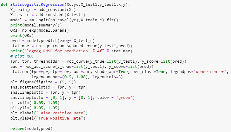
Statsmodels Output:

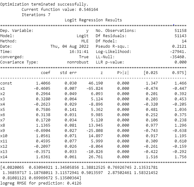
In this summary, you can see that → ‘euribor3m’,’default_unknown’,’month_may’, and ’day_of_week_mon’ these variables are negatively affecting customer conversion. Other variables are positively affected. In the fourth column, P>|z| shows the p-value, you can see that for all the variables, their values are less than 0.05, which means they are statistically significant.

You can see that AUC is greater than 0.5, which means the classifier is able to distinguish between converted customers and not converted customers.

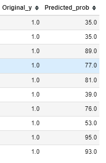
Here you can see that it’s generating probability converted customer class.

Now, if business people want to understand how confident we are when we say XYZ customer is going to get converted, you can use Statsmodel a which gives you probability if not you can use the Scikit-learn model for prediction.

Model Interpretation

Now, I’m putting customers into 3 buckets based on predicted probability →

1. Cold Lead: Customers who haven’t shown any interest in your ‘term deposit’ product. One of the most difficult leads to convert.
2. Warm Lead: Customers who are familiar with the way your business work or with ‘term deposit’ products. These customers engage in a conversation, so they are easier to a prospect than cold leads.
3. Hot Lead: Customers who have shown interest in your company or products. These leads require immediate attention because their interest may fade when you take too long to respond.

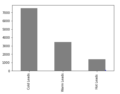
Now you have 3 buckets of potential leads, which you can pass on to the Sales team to work on. Sales and distribution teams can now create strategies on how to reach out to these Hot leads and acquire them.

Give it a clap if you found it informative. Comment if you have any suggestions 🙂

---

A guide to Predictive Lead Scoring using Machine Learning was originally published in Towards AI on Medium, where people are continuing the conversation by highlighting and responding to this story.

Join thousands of data leaders on the AI newsletter. It’s free, we don’t spam, and we never share your email address. Keep up to date with the latest work in AI. From research to projects and ideas. If you are building an AI startup, an AI-related product, or a service, we invite you to consider becoming a sponsor.

Published via Towards AI