K-Nearest Neighbors (KNN) Algorithm Tutorial — Machine Learning Basics

Diving into K-nearest neighbor, a fundamental classical machine learning (ML) algorithm

Acknowledgments: This work has been led by Sujan Shirol, supervised by Husna Sayedi, reviewed and edited by Roberto Iriondo. We used natural language optimization to improve the experience and sentiment of this article to our readers. Please let us know if you have any feedback on whether you would like to see more of this optimization. All images are from the author(s) unless stated otherwise.

The k-nearest neighbor algorithm, commonly known as the KNN algorithm, is a simple yet effective classification and regression supervised machine learning algorithm. This article will be covering the KNN Algorithm, its applications, pros and cons, the math behind it, and its implementation in Python. Please make sure to check the entire implementation from this tutorial on either Google Colab or Github to aid with your reading.

Let’s understand what is meant by classification and regression: classification is hardwired since we were kids. While the first-word we might have said would be either ‘dad’ or ‘mom.’ How would a baby know who their ‘mom’ or ‘dad’ is? We may have seen the video or heard from our parents how happy and excited they were to teach us how to identify them. They used to point at each other every day until we understood the difference.

Consequently, this method wherein pointing at each other to make us learn is known as supervised learning. Fundamentally, supervised learning is learning a function that maps an input to an output based on examples, input-output pairs [9].

The features by which a baby classifies are most likely to be the facial hair and voice, these are known as dependent variables/input, and the independent variable/output is binary, pretty much yes or no. This entire process can be called model training, and we will learn more sophisticated ways to implement this process in a way that the machines can understand. Similarly, when the independent variable/output is a constant value, it is known as a regression problem.

What is the K-Nearest Neighbors (KNN) Algorithm?

The KNN algorithm is a major classical machine learning algorithm that focuses on the distance from new unclassified/unlabeled data points to existing classified/labeled data points. Think of it as the process of entering a college in the middle of an academic year for whatever reason. As we can see, there may be already like-minded groups formed by the students among themselves, and it is just a matter of time for us to figure out what group we would fit in — particularly, which group we would feel more connected to, or in other words, less distanced from.

We already have labeled data points from our dataset. We will plot them on a 2-dimensional graph; these data points belong to three categories represented by red, green, and yellow colors, as shown in figure 1.

Next, we will consider a new unlabelled data point represented by the black cross mark. Making it time to determine which category this new data point belongs to from the three colors. First, we take a random value, which is known to be the k-value. The k-value tells the number of nearest points to look for from the new unlabelled data point. Consider the k-value as 5. Next, we calculate the distance from the unlabelled data point to every data point on the graph and select the top 5 shortest distances.

Amongst the top 5 nearest data points, 3 belong to category red, 1 belong to category green, and 1 belong to category yellow. These are known as k(5) nearest neighbors of new data. It is now evident that the new data point belongs to category red as most of its nearest neighbors are from category red.

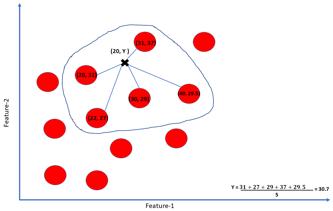
Similarly, in a regression problem, the aim is to predict a new data point’s value, not the category to which it belongs. Again, to illustrate, plot a 2-dimensional graph consisting of data points from the given dataset. Since it is a 2-dimensional graph, there are 2 features for each data point. The x-axis represents feature-1, and the y-axis represents feature-2.

Next, we introduce a new data point for which only the feature-1 value is known, and we need to predict the feature-2 value. We take a k-value of 5 and get the 5 nearest neighboring points from the new data point. The predicted value of feature-2 for the new data point is the mean of the feature-2 of 5 nearest neighbors.

When to use KNN?

1. The KNN algorithm can compete with the most accurate models because it makes highly accurate predictions. Therefore, we can use the KNN algorithm for applications that require high accuracy but that do not require a human-readable model [11].
2. When the provided dataset for our task is small.
3. When data is labeled correctly, and the predicted value will be among the given labels. If there is category 1, category 2, and category 3, then the predicted category should be one of them, not any other category.
4. KNN is used to solve regression, classification, or search problems

Pros and Cons of Using KNN

Pros

• It is straightforward and easy to implement the algorithm since it requires only two parameters: k-value and distance function.
• A good value of k will make the algorithm robust to noise.
• It learns a nonlinear decision boundary.
• There are almost no assumptions on the given data. The only thing that is assumed is nearby/similar instances belong to the same category.
• It is a non-parametric approach. No model fitting/training is required. The data speaks for itself.
• Since model training is not required, it is easy to update the dataset.

Cons

• Inefficient for large datasets since distance has to be calculated throughout every point, looping every time the algorithm encounters a new data point.
• KNN assumes similar data points are close to each other. Therefore, the model is susceptible to outliers. A few outliers from a particular category can draw the new data towards it even in cases when the new data belongs to a different category.
• It cannot handle imbalanced data. When the data is imbalanced, there is a lot more data belonging to one particular category than the rest of the categories; the algorithm will be biased. Therefore, it needs to be handled explicitly.
• If our dataset requires a K that is a large number, it will increase the computational expense of the algorithm.

Diving Into the Math Behind KNN

As discussed, the algorithm calculates the distance from the new data point to each existing data point. The question is, how is the distance measured? There are three methods, which we will discuss in this work.

Minkowski Distance:

a) The Minkowski Distance is a generalized distance function in a normed vector space. The vector space must meet the following requirements:

1. Zero Vector: The vector zero has 0 length
2. Scalar Factor: Multiplying a vector with a scalar only changes the length, not the direction
3. Triangle Inequality: The shortest distance between any two given points is a straight line.

b) In cases,

1. When p=1 — this is the Manhattan Distance
2. When p=2 — this is the Euclidean Distance
3. When p=infinity — this is the Chebyshev Distance

Euclidean distance

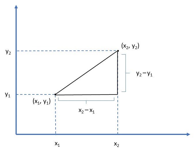
In mathematics, the Euclidean distance between two points in the Euclidean space is the line segment’s length between the two points. It can be calculated from the points’ cartesian coordinates using the Pythagorean theorem, therefore occasionally being called the Pythagorean distance [10].

To calculate the distance between two points (x1, y1) and (x2, y2) on a 2-dimensional plane, we use the following formula:

Manhattan distance

The Manhattan distance calculation is similar to the calculation of Euclidean distance, with the only difference being that we take absolute value instead of taking the square root of the sum of squared difference. By taking the absolute value, we are not calculating the shortest distance between two points like in a Euclidean distance.

Fundamentally, the Euclidean distance represents “flying from one point to another,” and the Manhattan distance is “traveling from one point to another point” in a city following the pathway or the road.

However, and most likely, the method used to calculate distance is the Euclidean distance formula. One of the reasons being, Euclidean distance can calculate the distance in any dimension, whereas Manhattan finds the elements on a vertical or a horizontal plane.

How to Choose the Right Value for K?

Choosing K is unique to every dataset. There is no standard statistical method to compute the most optimal K value. We want to choose a K value that will reduce errors. As we increase K, our predictions become more stable due to averaging or majority voting. However, if K is too large, then the error rate will increase again as it will underfit the model. In other words, a small K yields a low bias and high variance (higher complexity), while a large K yields a high bias and a low variance. That being said, there are few different methods to try:

1. Domain knowledge: As noted previously, K is highly data-dependent. For example, if one analyzes a distinct flower species dataset, it is easy to see that K should be that specific number of flower species.
2. Cross-Validation: This well-known technique is useful in comparing accuracy measures of a range of K values, e.g., K being values from 1 to 10. This technique entails breaking the training set into test/validation sets to tune K to find the optimal value.
3. Square Root: A simple method to try when one has little domain knowledge about the data is to square root the number of data points in the training set.

Implementation of KNN in Python

For the implementation of the KNN algorithm, we will be using the Iris dataset. The Iris dataset is a collection of morphologic variations of Iris flowers of three related species: Setosa, Versicolor, Virginica. The observed morphologic variations are sepal length, sepal width, petal length, and petal width.

Sklearn is a Python library that features various classification, regression, and clustering algorithms. It also holds the Iris dataset as sample data. We will import necessary libraries like NumPy, Pandas, and matplotlib.

import numpy as np
import pandas as pd
import matplotlib.pyplot as plt
import seaborn as sns
from sklearn.model_selection import train_test_split
from sklearn.neighbors import KNeighborsClassifier
from sklearn.model_selection import cross_val_score
from sklearn.datasets import load_iris
iris = load_iris()

The table below shows how the first 5 rows of data look like once we have it in a Pandas DataFrame. The target values are 0.0, 1.0, and 2.0, representing Setosa, Versicolor, and Virginica, respectively.

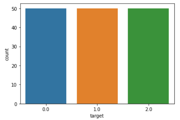
Since KNN is sensitive to outliers and imbalanced data, checking for the same and handling it is very important. Checking for imbalance data by plotting a count plot for the target variable, there are 50 samples of each flower type. Consequently, the data is perfectly balanced.

sns.countplot(x=’target’, data=iris)

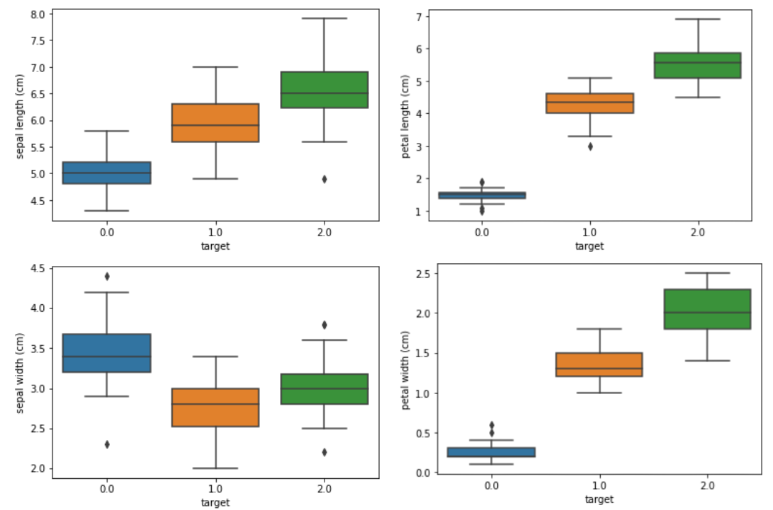
By checking for outliers using boxplot, there seem to be not many outliers to be handled.

for feature in [‘sepal length (cm)’, ‘sepal width (cm)’, ‘petal
 length (cm)’, ‘petal width (cm)’]:
sns.boxplot(x=’target’, y=feature, data=iris)
plt.show()

Next, we split the data into training and testing sets to measure how accurate the model is. The model will be trained on the training set, which is randomly selected 60% of the original data and then evaluated with a testing set which is the remaining 40% of the original data. Before splitting it into training and testing sets, it is essential to separate the feature/dependent and target/independent variable.

X = iris.drop([‘target’], axis=1)
y = iris[‘target’]
X_train, X_test, y_train, y_test = train_test_split(X, y, test_size=0.4, random_state=0)

Building the initial model with a k-value of 1, meaning only 1 nearest neighbor will be considered for classifying a new data point. Internally, the distance from the new data point to all the data points will be calculated and then sorted from smallest to largest, along with their respective classes. Since the k-value is 1, the class (target value) of the first instance from the sorted array will determine the new data class. As we can see, we obtain a decent accuracy score of 91.6%. However, the optimal k-value needs to be selected.

knn = KNeighborsClassifier(n_neighbors=1)
knn.fit(X_train, y_train)
print(knn.score(X_test, y_test))
Output: 0.9166666666666666

To find the optimal k-value by cross-validation method, we calculate the k-values’ accuracy ranging from 1 to 26 in this case and choosing the optimal k-value. The accuracy score ranges between 86% to 96% approximately. As observed, the accuracy score starts from a low value, reaches a peak at some point, stays approximately constant for a while, and then again drops. The range where the score remains constant for some time can be considered as an optimal k-value for the given dataset.

k_range = list(range(1,26))
scores = []
for k in k_range:
knn = KNeighborsClassifier(n_neighbors=k)
knn.fit(X_train, y_train)
y_pred = knn.predict(X_test)
scores.append(metrics.accuracy_score(y_test, y_pred))
plt.plot(k_range, scores)
plt.xlabel(‘Value of k’)
plt.ylabel(‘Accuracy Score’)
plt.title(‘Accuracy Scores for different values of k’)
plt.show()

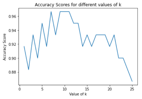
Introducing a new unlabeled data point whose class we need to predict is the flower type, which belongs to a category based on its morphologic features. We will build the model with a k-value of 11.

knn = KNeighborsClassifier(n_neighbors=11)
knn.fit(iris.drop([‘target’], axis=1), iris[‘target’])
X_new = np.array([[1, 2.9, 10, 0.2]])
prediction = knn.predict(X_new)
print(prediction)
if prediction[0] == 0.0:
print(‘Setosa’)
elif prediction[0] == 1.0:
print(‘Versicolor’)
else:
print(‘Virginica’)
Output: [2.]
Virginica

KNN Applications

From forecasting epidemics [2] and the economy to information retrieval [4] [5], recommender systems [3], data compression, and healthcare [1], the k-nearest neighbors (KNN) algorithm has become fundamental in such applications. KNN is known for being one of the most straightforward supervised machine learning algorithms, and its implementations are primarily used during regression and classification tasks, as we have discussed.

One of the most significant use cases for the k-nearest neighbor algorithm is recommendation systems [3] [6]. A simple Google search gives us several promising articles to implementations on recommender systems using KNN [7], mainly due to KNN’s ability to propagate similar recommendations for a set of particular items.

For instance, imagine that we put a group of users with a diverse and pseudorandom interest in movies. A recommendation system compares the users’ profiles to find whether a set of users has a similar taste. Afterward, suppose two users have a similar taste on two or more items during the comparison. In that case, an item that the first user enjoys might probably be enjoyable to the second user.

Similarly, KNN can be of use during classification tasks [8].

Conclusion

KNN is a highly effective, simple, and easy-to-implemented supervised machine learning algorithm that can be used for classification and regression problems. The model functions by calculating distances of a selected number of examples, K, nearest to the predicting point.

For a classification problem, the label becomes the majority vote of the nearest K points. For a regression problem, the label becomes the average of the nearest K points. Whenever a prediction is being made, the model searches the entire training set to find the K-most similar examples to label the original prediction point.

The major drawback to this algorithm is that as the number of data increases, so does the computational expense and time. However, if the dataset we are working with is a proper size dataset (like the Iris dataset), KNN is an easy and straightforward algorithm to implement as there is no need to build a model, tune parameters, or make any additional assumptions on the model.

DISCLAIMER: The views expressed in this article are those of the author(s) and do not represent the views of any company (directly or indirectly) associated with the author(s). This work does not intend to be a final product, yet rather a reflection of current thinking, along with being a catalyst for discussion and improvement.

All images are from the author(s) unless stated otherwise.

Published via Towards AI

Resources

Youtube Tutorial.

References

[1] Prediction of COVID-19 Possibilities using KNN Classification Algorithm, (2021). Retrieved 14 January 2021, from https://assets.researchsquare.com/files/rs-70985/v2_stamped.pdf

[2] Prediction Model for Influenza KNN Algorithm Based Classification on Twitter Data, Kavitha, et al., (2021). Retrieved 14 January 2021, from http://ijseas.com/volume1/v1i7/ijseas20150712.pdf

[3] Subramaniyaswamy, V., & Logesh, R. (2017). Adaptive KNN based Recommender System through Mining of User Preferences. Wireless Personal Communications, 97(2), 2229–2247. DOI: 10.1007/s11277–017–4605–5

[4] Introduction to Information Retrieval, Chris Manning and Pandu Nayak, Stanford University, (2021). Retrieved 14 January 2021, from https://web.stanford.edu/class/cs276/handouts/lecture12-textcat.pdf

[5] Nearest neighbor search. (2021). Retrieved 14 January 2021, from https://en.wikipedia.org/wiki/Nearest_neighbor_search

[6] Recommendation System Based on Collaborative Filtering, Zheng Wen, Stanford University, (2021). Retrieved 14 January 2021, from http://cs229.stanford.edu/proj2008/Wen-RecommendationSystemBasedOnCollaborativeFiltering.pdf

[7] recommendation systems using KNN — Google Search. (2021). Retrieved 14 January 2021, from https://mktg.best/a1t-9

[8] K-nearest neighbors algorithm. (2021). Retrieved 14 January 2021, from https://en.wikipedia.org/wiki/K-nearest_neighbors_algorithm

[9] “Supervised Learning”. 2021. En.Wikipedia.Org. https://en.wikipedia.org/wiki/Supervised_learning#cite_note-1.

[10] ”Euclidean Distance”. 2021. En.Wikipedia.Org. https://en.wikipedia.org/wiki/Euclidean_distance#:~:text=In%20mathematics%2C%20the%20Euclidean%20distance,being%20called%20the%20Pythagorean%20distance.

[11] “IBM Knowledge Center”. 2021. Ibm.Com. https://www.ibm.com/support/knowledgecenter/SSCJDQ/com.ibm.swg.im.dashdb.analytics.doc/doc/r_knn_usage.html.

Metadata: {knn algorithm} {knn classifier} {knn in r} {knn in python} {sklearn knn} {knn regression} {knn clustering} {knn classifier sklearn} {knn supervised} {knn classification} {knn vs k means} {knn algorithm example} {knn overfitting}