Spoken Language Recognition Using Convolutional Neural Networks

Last Updated on December 17, 2020 by Editorial Team

Author(s): Joscha Simon Rieber

Automatically identify the spoken language from a speech audio signal with TensorFlow

Introduction

Applications

At Fraunhofer IAIS, we work on various speech technologies such as automatic speech recognition, speaker recognition, etc. In recent work, I developed a new service predicting the spoken language directly from the audio stream. If the language is known, a suitable model for the speech recognition step can be selected automatically. Potential applications for this can be automatic transcription software and conversational AI.

Open-Source Code

I have prepared a GitHub repository including Jupyter Notebooks that can be used to experiment and train an own spoken language recognizer. In the current state, it is capable of distinguishing between German and English. You can see this as a starting point to implement your own language recognizer. We are mainly using Python 3, TensorFlow 2, and librosa.

Approach

The concept is based on publications by Bartz et. al [1] and Sarthak et. al [2], who are utilizing convolutional neural networks (CNN) to implement spoken language identification systems. The idea is to analyze the spectrogram of a short audio segment containing a speech signal with a huge CNN for classification. We are using the Mel-scaled spectrogram similar to Pröve [4].

Results

The open-source variant of my language recognition based on Common Voice data yields an accuracy of 93.8 % classifying English and German. At our institute, we are using our own media datasets and obtain an overall accuracy of 98.2 % with the same code tested on 152 h of augmented testing data. Our algorithm can distinguish between English, German, and “other” (unknown class).

Dataset

The dataset used in the notebooks is based on Mozilla’s Common Voice. You will need to download the English and the German datasets and then run the scripts from the first notebook to extract a training and an evaluation dataset containing speech signals with a duration between 7.5 and 10 seconds.

Data Augmentation

The training dataset can be augmented by adding noise. This will later help to improve the robustness of the final model against noise affected recordings. We use the Numpy function random.normal for a normal (Gaussian) distribution, which gives us white noise.

def add_noise(audio_segment, gain):
    num_samples = audio_segment.shape[0]
    noise = gain * numpy.random.normal(size=num_samples)
    return audio_segment + noise

Data Preprocessing

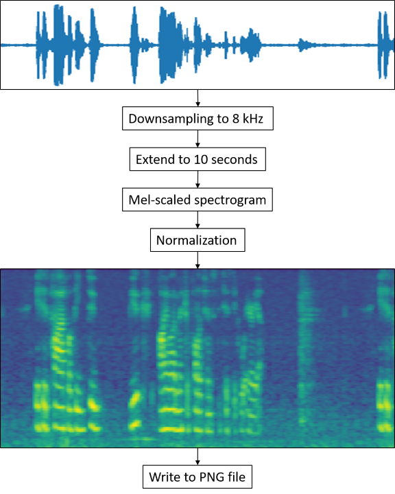
All audio files are preprocessed to extract a Mel-scaled spectrogram. This is done with the following steps.

Loading the Audio File

def load_audio_file(audio_file_path):
    audio_segment, _ = librosa.load(audio_file_path, sr=sample_rate)
    return audio_segment

In this step, the audio is loaded and downsampled to 8 kHz to limit the bandwidth to 4 kHz. This helps to make the algorithm robust against noise in the higher frequencies. As stated in [1], most of the phonemes in the English language do not exceed 3 kHz.

Fixing the Duration to 10 Seconds

def fix_audio_segment_to_10_seconds(audio_segment):
    target_len = 10 * sample_rate
    audio_segment = numpy.concatenate([audio_segment]*2, axis=0)
    audio_segment = audio_segment[0:target_len]
    
    return audio_segment

We duplicate the signal that is between 7.5 and 10 seconds long and cut it to 10 seconds.

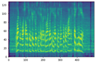
Mel-scaled Spectrogram

The Mel-scaled spectrogram is computed from the audio. It helps analyzing the speech frequencies with the neural network. The Mel-scaling represents lower frequencies with a higher resolution than higher frequencies and takes into account the way humans perceive frequencies.

def spectrogram(audio_segment):
    # Compute Mel-scaled spectrogram image
    hl = audio_segment.shape[0] // image_width
    spec = librosa.feature.melspectrogram(audio_segment,
                                     n_mels=image_height, 
                                     hop_length=int(hl))

    # Logarithmic amplitudes
    image = librosa.core.power_to_db(spec)

    # Convert to numpy matrix
    image_np = numpy.asmatrix(image)

    # Normalize and scale
    image_np_scaled_temp = (image_np - numpy.min(image_np))
    
    image_np_scaled = image_np_scaled_temp / 
                      numpy.max(image_np_scaled_temp)

    return image_np_scaled[:, 0:image_width]

Normalization takes place to adjust the values in the spectrogram between 0 and 1. This step equalizes quiet and loud recordings to a common level.

Conversion to PNG

All files are finally stored as PNG files of size 500 x 128, but first, the normalized spectrograms need to be converted from decimal values between 0 and 1 to integer values between 0 and 255.

def to_integer(image_float):
    # range (0,1) -> (0,255)
    image_float_255 = image_float * 255.0
    
    # Convert to uint8 in range [0:255]
    image_int = image_float_255.astype(numpy.uint8)
    
    return image_int

Model Training

Accessing the Datasets

To make the datasets accessible for the model training algorithm, we first need to instantiate generators that iterate the datasets in a memory efficient way. This is important because we have 60,000 images for both training and evaluation data and we cannot just load it into memory. Fortunately, Keras, which is part of TensorFlow, has amazing functions to deal with image datasets. I am using the ImageDataGenerator as a data input source for the model training.

image_data_generator = ImageDataGenerator(
                                  rescale=1./255,      
                                  validation_split=validation_split)

train_generator = image_data_generator.flow_from_directory(
                        train_path,
                        batch_size=batch_size,
                        class_mode='categorical',
                        target_size=(image_height, image_width), 
                        color_mode='grayscale',
                        subset='training')

validation_generator = image_data_generator.flow_from_directory(
                            train_path,
                            batch_size=batch_size,
                            class_mode='categorical',
                            target_size=(image_height, image_width), 
                            color_mode='grayscale',
                            subset='validation')

A suitable batch-size is 128, which is big enough to help reducing over-fitting and keeps the model training efficient.

Model Definition Inception V3

As suggested in [1], a huge CNN such as Inception V3 is recommended to solve this task. Spoken language recognition is a very complex task that demands a model with a big capacity. Smaller networks perform worse because they are not capable of handling the complexity of the data.

The original Inception V3 model [3], which is already available from Keras Applications, must be slightly adapted to process our dataset. It is expected to process images with 3 different color layers, but our images are grayscale. The following lines of code copy the single image color layer to all three channels for the input tensor for Inception V3.

img_input = Input(shape=(image_height, image_width, 1))

img_conc = Concatenate(axis=3, name='input_concat')([img_input, img_input, img_input])

model = InceptionV3(input_tensor=img_conc, weights=None, include_top=True, classes=2)

The model has nearly 22 mio parameters.

Compiling the Model

model.compile(
         optimizer=RMSprop(lr=initial_learning_rate, clipvalue=2.0),       
         loss='categorical_crossentropy',
         metrics=['accuracy'])

In my evaluations, the RMS-Prop optimizer yielded good results. Adam is suggested in [1].

Early Stopping

Training can be speeded up by automatically stopping when the learning finishes. I use Keras’ EarlyStopping method to do so.

early_stopping = EarlyStopping(monitor='val_accuracy', mode='max', patience=5, restore_best_weights=True)

Learning Rate Decay

As suggested in [1], I implemented an exponential learning rate decay.

def step_decay(epoch, lr):
    drop = 0.94
    epochs_drop = 2.0
    lrate = lr * math.pow(drop, math.floor((1+epoch)/epochs_drop))
    return lrate

learning_rate_decay = LearningRateScheduler(step_decay, verbose=1)

Training

Now, the actual training takes place using the following command.

model.fit(train_generator,
          validation_data=validation_generator,
          epochs=60,
          steps_per_epoch=steps_per_epoch,
          validation_steps=validation_steps,
          callbacks=[early_stopping, learning_rate_decay])

The number of epochs is very high, but since I am using early stopping, fortunately, the algorithm stops after 36 epochs.

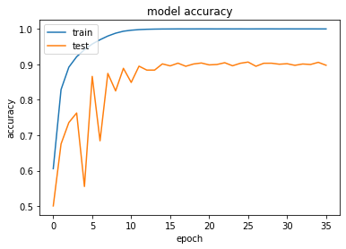
When looking at the training and evaluation accuracies for the 36 epochs, we can see that there is overfitting involved, which means that the model is much more accurate in classifying the training dataset than the evaluation dataset. This is due to the fact that the Inception V3 model is huge and has an enormous capacity. Using such a big network means that the amount of diverse training data should be very large, as well. So, to overcome this issue, you can increase the amount of training data up to the point where overfitting does not occur any more. In the plot, you can also see the effect of the learning rate decay. The steepest learning curve can be seen for the first 10 epochs.

Evaluation

Finally, I instantiate a new ImageDataGenerator for the testing data and use

_, test_accuracy = model.evaluate(evaluation_generator, 
                                  steps=evaluation_steps)

to evaluate the model. The result is a testing accuracy of 93.8 %.

Adapting and Improving the Model

Feel free to use the code to improve the model. For example, you can add more classes and feed it with more data from other languages. Also, it is recommended to adapt the data and the augmentation to your application. We at Fraunhofer have an optimized version trained on media data. We are using two additional augmentation steps to improve results on double-talk (overdub) and background music. You can also alter pitch and speed to perform data augmentation. Moreover, it is recommended to use much more data. If the amount and diversity of the training dataset is not sufficient, overfitting might occur.

Summary

I have introduced my open-source code on GitHub and the implemented approach for identifying the spoken language directly from speech audio. The model accuracy is 93.8 % for the given datasets based on Common Voice. The idea is to analyze the Mel-scaled spectrogram of a 10 seconds long audio segment using a CNN with a high capacity. Since language recognition is a complex task, the network needs to be large enough to capture the complexity and derive meaningful features during training. I suggest to further improve the model by extending the dataset and the augmentation techniques. Then, testing accuracies above 98 % are possible without changing the training implementation itself.

References

[1] C. Bartz, T. Herold,H. Yang and C. Meinel, Language Identification Using Deep Convolutional Recurrent Neural Networks (2015), Proc. of International Conference on Neural Information Processing (ICONIP)

[2] S. S. Sarthak, G. Mittal, Spoken Language Identification using ConvNets (2019), Ambient Intelligence, vol. 11912, Springer Nature 2019, p. 252

[3] C. Szegedy, V. Vanhoucke, S. Ioffe, J. Shlens and Z. Wojna, Rethinking the Inception Architecture for Computer Vision (2015), CoRR, abs/1512.00567

[4] P.-L. Pröve, Spoken Language Recognition (2017), GitHub Repository

Bio: Joscha Simon Rieber is a research engineer at Fraunhofer IAIS in Sankt Augustin, Germany. There, he works on a transcription system and conversational AI for the speech technologies team. Prior, Rieber was a software engineer and digital signal processing expert for Brainworx Audio GmbH. He studied computer science and achieved his master’s degree at the University of Bonn in Germany.

---

Spoken Language Recognition Using Convolutional Neural Networks was originally published in Towards AI on Medium, where people are continuing the conversation by highlighting and responding to this story.

Published via Towards AI