Image De-noising Using Deep Learning

Last Updated on January 6, 2023 by Editorial Team

Last Updated on January 23, 2021 by Editorial Team

Author(s): Chintan Dave

Computer Vision, Deep Learning

Denoising an image is a classical problem that researchers are trying to solve for decades. In earlier times, researchers used filters to reduce the noise in the images. They used to work fairly well for images with a reasonable level of noise. However, applying those filters would add a blur to the image. And if the image is too noisy, then the resultant image would be so blurry that most of the critical details in the image are lost.

There has to be a better way to solve this problem. As a result, I have implemented several deep learning architectures that far surpass the traditional denoising filters. In this blog, I will explain my approach step-by-step as a case study, starting from the problem formulation to implementing the state-of-the-art deep learning models, and then finally see the results.

Contents Summary

1. What is noise in images?
2. Problem Formulation
3. Machine Learning Problem Formulation
4. Source of Data
5. Exploratory Data Analysis
6. An Overview on Traditional Filters for Image Denoising
7. Deep Learning Models for Image Denoising
8. Results Comparison
9. Deployment
10. Future Work and Scope for Improvement
11. References

1. What is noise in images?

Image noise is a random variation of brightness or color information in the images captured. It is degradation in image signal caused by external sources. Mathematically, noise in an image can be represented by,

A(x,y) = B(x,y) + H(x,y)

Where,

A(x,y)= function of noisy image;
B(x,y)= function of original image;
H(x,y)= function of noise;

To understand more about noise, check out this blog.

2. Problem Formulation

Traditional image denoising algorithms always assume the noise to be homogeneous Gaussian distributed. However, in practice, the noise on real images can be much more complex. Such noise on real images is called Real-noise or Blind-noise. Traditional filters fail to perform well on images with such noise.

So, the problem formulation becomes,

How can we denoise images containing blind noise?

Objective and Constraints

• The goal is to denoise the color images with blind noise
• No latency constraint, because I would like to denoise the images as close to the ground truth as possible, even if it takes a reasonable amount of time

The term blind denoising refers to the fact that the basis used for denoising is learned from the noisy sample itself during denoising. In other words, whatever deep learning architecture we build should learn the noise distribution in the images inherently and denoise it. So as always, it all depends on the type of data we provide to the deep learning model.

3. Machine Learning Problem Formulation

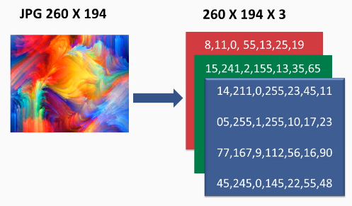
First, let us consider the format of an RGB image.

Any RGB image has three color channels – Red, Green, and Blue, for each pixel.

Now, each color is represented by an 8-bit number which has a range of 0–255. So, any image can be represented by a 3-dimensional matrix.

Now consider the same thing for a noisy image.

We saw in the earlier section that noise is a random variation in the pixels. In other words, some of the pixels’ numeric values for the 3 channels in the image is corrupted. To restore the image to its original form, we need to rectify those corrupted pixel values.

Type of Machine Learning problem

• We can look at this as a supervised learning regression problem, where we are predicting the true value of the corrupted pixel [number in the range of 0–255].

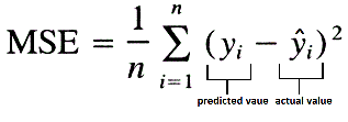
Loss function and Performance Metric

• The loss that I will be using is MSE (Mean Squared Error). The lower the score better it is.

• For performance evaluation, I will be using two metrics,
  PSNR (Peak Signal to Noise Ratio)
  SSIM (Structural Similarity Index Measure)
  For both, the higher the score better it is.

4. Source of Data

As this is a supervised learning problem, we need the pair of noisy images (x) and ground truth images (y).

I have collected the data from three sources.

1. SIDD — Contains 160 pairs of [Noisy – Ground truth] images from the smartphone camera
2. RENOIR — Contains 80 pairs [Noisy — Ground truth] images from the smartphone camera
3. NIND — Contains 62 pairs of [Noisy — Ground truth] images from Fujifilm X-T1 DSLR camera

5. Exploratory Data Analysis

Analysis of the meta-data

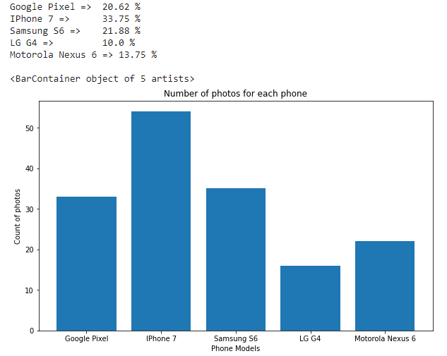
We can see that majority of the photos have been clicked on iPhone 7, followed by Samsung S6 and Google Pixel. LG G4 has the least number of photos.

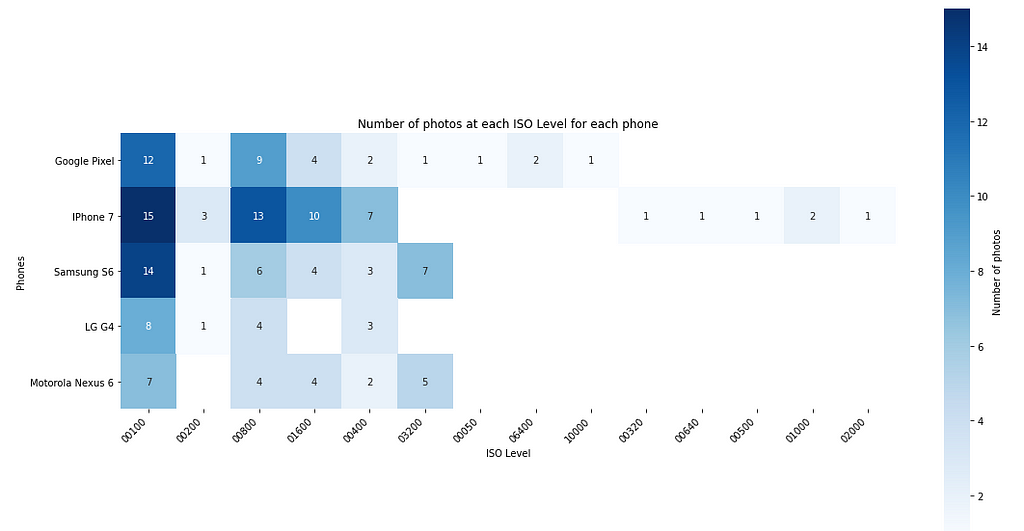
There are a total of 14 unique ISO level settings used in the dataset. Most of the photos are clicked at a low ISO setting. The most used ISO settings are 100 and 800 followed by 1600,400 and 3200. The higher the exposure, the brighter the image will be and vice-versa.

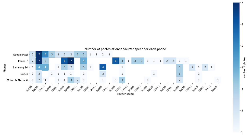
Most of the photos are clicked at 100 shutter speed, followed by 400 and 800. The higher the shutter speed darker the image will be, and vice-versa.

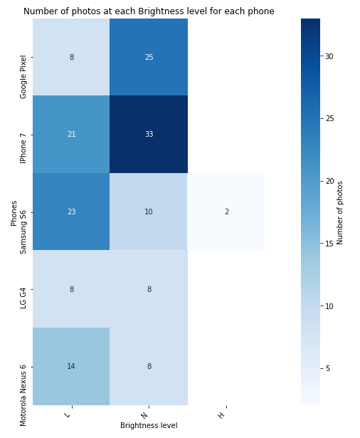
The majority of the photos are clicked in Normal brightness mode, followed by Low brightness. Only 2 photos are clicked at High brightness on Samsung S6.

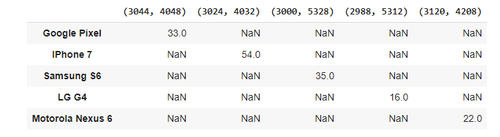
We can see each phone has its own image resolution. Every individual phone captured photos with the same resolution.

Analysis of the Image data

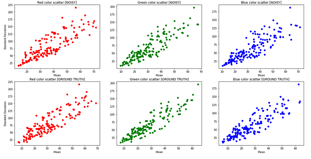
It is seen that most of the mean pixel values are at a lower to medium value (darker to medium brightness images). Only a few of them are very high value(bright images). You can also see some means in the noisy images have differences as compared to the ground truth images. The difference is more easily visible at higher pixel values.

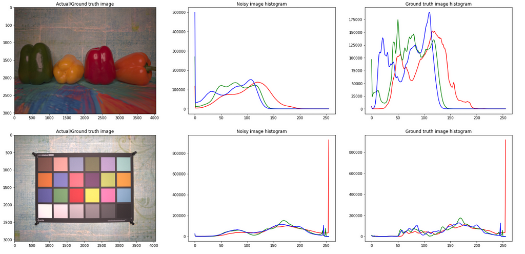
It can be observed that the noisy images have a smooth distribution of pixel intensity as compared to the original images. The reason for this is that, whenever there is noise in an image, the camera has failed to capture the color info for those pixels (due to various reasons), and hence, to fill the ‘no color’ in those pixels, mostly it fills with some random value by the camera software. Due to these random values (noise) the pixel values get smoothed out.

6. An Overview on Traditional Filters for Image Denoising

Traditionally, researchers came up with filters to denoise an image. Most of the filters were specific to the type of noise the image has. There are several types of noises like Gaussian noise, Poisson noise, Speckle noise, Salt and Pepper noise, etc. There are specific filters for each type of noise. Hence, the first step to denoise an image using traditional filters is to identify the type of noise present in the image. After identifying that, we can go ahead and apply the specific filter. To identifying the type of noise, there are certain mathematical formulas to help us guess the type of noise. Or else a domain expert can decide it just by looking at the image. There are also some filters that work on any type of noise.

There are tons of filters available for denoising an image. All have their pros and cons. Here, I will be discussing the Non-Local Means (NLM) algorithm which is seen to be working very well to denoise an image.

Non-Local Means

First, let me show you the formula for NLM,

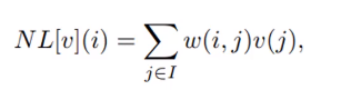
The algorithm calculates the estimated value of a pixel as the weighted average of all the pixels in the image, but the family of weights depends on the similarity between the pixels i and j. In other words, it looks at a patch of image and then identifies other similar patches in the whole image and takes a weighted average of them. To understand this, consider the following image,

Here, similar patches are marked with the same colored square boxes. So now, it will take the weighted average of pixels of similar patches as the estimated value of the target pixel. This algorithm takes as input the patch size and the patch distance.

Consider the following grayscale image which has been denoised using an NLM filter.

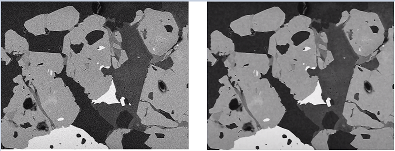
You can see that NLM does a decent job of denoising an image. If you look closely, then you will notice a slight blur to the denoised image. This is because of the mean. A mean applied to any data will smooth out the values.

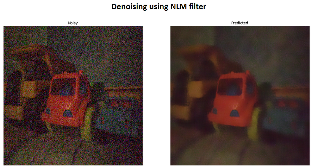
However, when the level of noise is too high, NLM fails to provide good results. Consider the following image which has been denoised using NLM filter.

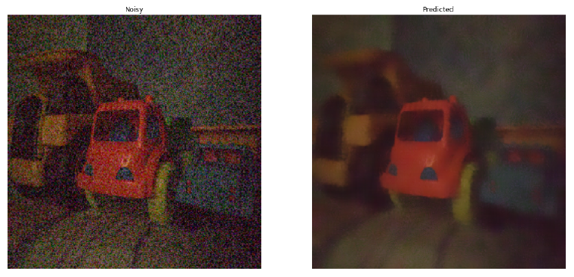
You can clearly see that after denoising, the image is too blurry and most of the critical details are lost in it. For example, observe the orange headlights in the blue truck.

7. Deep Learning Models for Image Denoising

With the advent of Deep Learning techniques, it is now possible to remove the blind noise from images such that the result is very close to the ground truth images with minimal loss of detail.

I have implemented three deep learning architectures,

1. REDNet
2. MWCNN
3. PRIDNet

REDNet — Residual Encoder-Decoder Networks

This is a CNN based auto-encoder architecture with skip connections. The architecture is as follows,

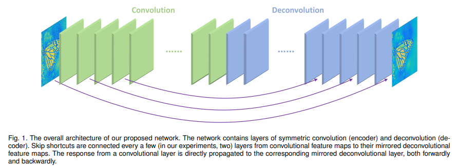
Here, I have used 5 layers of Convolution for the encoder and 5 layers of Deconvolution for the decoder. This is quite a simple architecture, which I used as a baseline.

I have shared my full code for REDNet on my Github repo.

Results

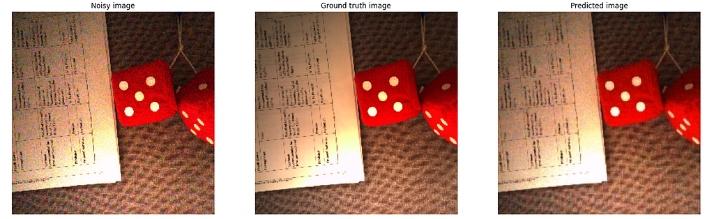
As you can see that this architecture is working fairly well in denoising the image. You can definitely see some reduction in the noise, and the image is trying to adapt to the original colors of the image for the corrupted pixels.

This architecture gave a PSNR score of 30.5713 and an SSIM score of 0.7932.

MWCNN — Multi-level Wavelet CNN

This is a wavelet-based deep learning architecture. Its architecture has a striking similarity with a U-Net architecture. The only difference in MWCNN is that, unlike down-sampling and up-sampling in U-Net, here we use DWT (Discrete Wavelet Transform) and IWT (Inverse Wavelet Transform). How the DWT and IWT work is beyond the scope of this blog. However, I have attached few resources [in the References section] from where you can learn it.

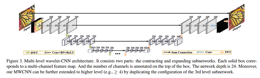
Here, I have extended this architecture up to 4 levels. So my network depth becomes 32. The code for this is a bit long and I have made use of custom layers in Keras. You can check out my full code for MWCNN on my Github repo.

Results

We can see that this architecture is working way better and the image is clearer as compared to REDNet.

This architecture gave a PSNR score of 32.5221 and an SSIM score of 0.8397.

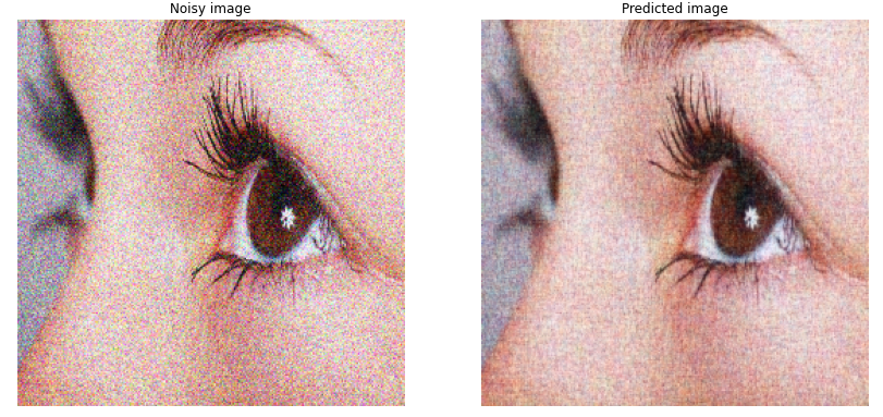
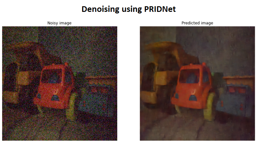
PRIDNet — Pyramid Real Image Denoising Network

This is a state-of-the-art deep learning architecture for blind denoising. This architecture is not as straight forward as we saw in the earlier two networks. PRIDNet has several modules, which are divided into three main parts.

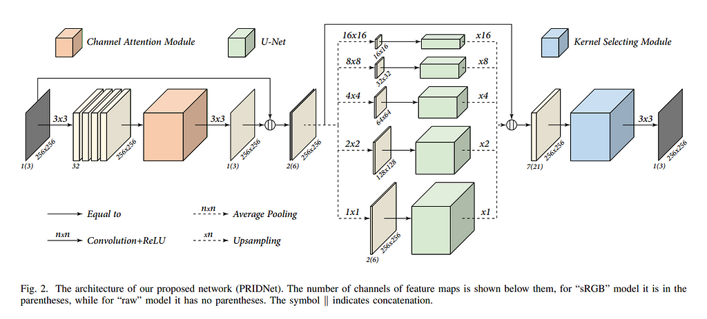
It might seem a bit overwhelming at first. But let me break it down into pieces. Trust me it is very easy to understand.

Channel Attention Module

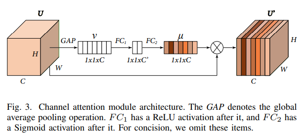
The Channel Attention module is responsible for the attention mechanism. Here, the attention mechanism is implemented in such a way that, it will put attention on each channel of the input U. Now, this “attention” can be thought of as weights. So there will be one weight for each channel. As a result, the attention weights will be a vector of size C [number of channels]. This vector will be multiplied to the input U. As we want to “learn” the attention, we will need this vector to be trainable. So the process that PRIDNet implements is that first we do a Global Average Pooling on the input and then pass it from 2 Fully Connected layers, the result of which should be a vector with the number of channels. These are the attention weights μ.

Multi-Scale Feature Extraction Module / Pyramid Module

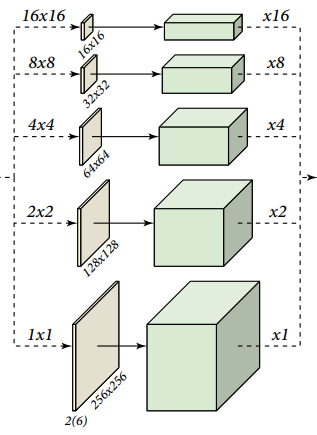
This is the heart of the whole architecture. Here, first, we will apply Average Pooling with the given kernel sizes. This will down-sample the image. Then we will apply a U-Net architecture to it. I chose to have 5 levels of deep U-Net. Finally, we will do Up-sampling with the same size as we did in Average Pooling. So, this will restore the image to the same size as the input (input to this module).

We will do this 5 times with different kernel sizes, and then finally we will concatenate the results.

Kernel Selecting Module

This module is inspired by a research paper that introduced Selective Kernel Networks. The idea behind this network is very well articulated by the research paper as follows,

In standard Convolutional Neural Networks (CNNs), the receptive fields of artificial neurons in each layer are designed to share the same size. It is well-known in the neuroscience community that the receptive field size of visual cortical neurons are modulated by the stimulus, which has been rarely considered in constructing CNNs.

A building block called Selective Kernel (SK) unit is designed, in which multiple branches with different kernel sizes are fused using softmax attention that is guided by the information in these branches. Different attentions on these branches yield different sizes of the effective receptive fields of neurons in the fusion layer.

This module is very similar to the Channel Attention module. As per the PRIDNet paper, the resultant vectors α, β, γ of size C denotes soft attention for U’, U’’ and U’’’ respectively.

An easy to grasp bird’s-eye-view diagram of the whole PRIDNet architecture is as follow,

I have shared my full code for PRIDNet on my Github repo.

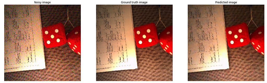
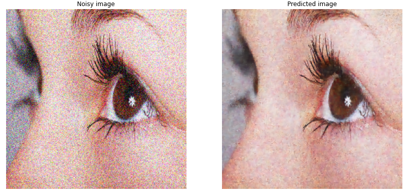
Results

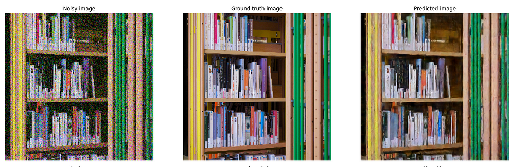
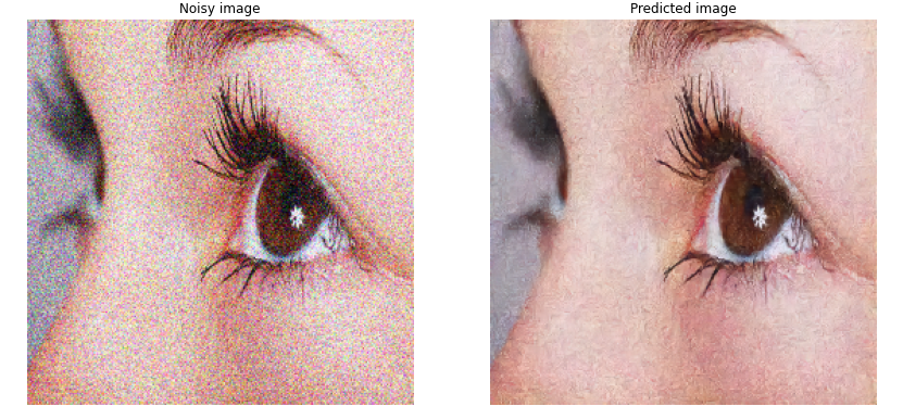
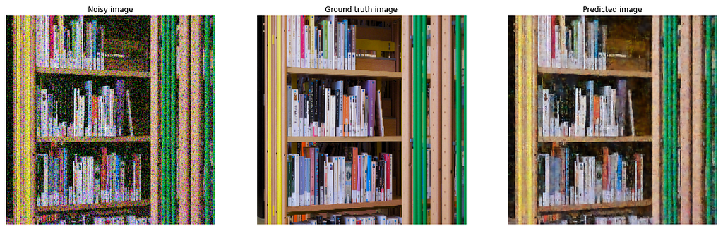
You can see that this architecture is giving the best results as compared to the previously discussed architectures. In the above close-up image of the eye, notice the level of detail in the eyeball in the denoised image!

Also, check out the Library image above. I have cropped a portion of it below,

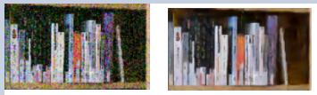
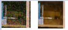
Notice the books with black color in the noisy image [Cropped Library books]. They are almost indistinguishable from the surrounding brown furniture. It all seems to be black. However, our model is able to denoise it in such a way that it can at least distinguish the books and the surrounding furniture. The same goes with the second image [Cropped Library furniture]. In its noisy image, you can see that the furniture has very dark, and it seems to be almost black on top. However, our model is able to understand the brown color and denoise it accordingly. How amazing is this!

This architecture gave a PSNR score of 33.3105 and an SSIM score of 0.8534.

8. Results Comparison

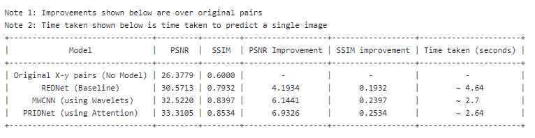
We can clearly see that PRIDNet is the best performing architecture with the least amount of time consumed to denoise a single image.

Now let’s compare the results of the NLM filtering and PRIDNet.

Critical areas to compare,

• The roof area of the yellow truck
• The seat of the orange truck
• The orange headlights in the blue truck
• The roof of the blue truck (observe the shadow)
• The two thin stripes in the middle of the floor
• The list can go on and on!

9. Deployment

I have created a Web-app using Streamlit and deployed the same. As of now, I have deployed it on localhost, because my model sizes are too big to be uploaded and used into memory on free cloud resources like Heroku, GCP App Engine, AWS EC2, Azure Web app, etc. However, I am looking for workarounds. Stay tuned for any updates here!

Meanwhile, check out the video demo of my Web-app,

10. Future Work and Scope for Improvement

Image denoising is an active field of research and every now and then there are amazing architectures being developed to denoise the images. Recently, researchers are using GANs to denoise images, which has proven to give some amazing results. A good GAN architecture will definitely improve the denoising further.

11. References

• https://medium.com/image-vision/noise-in-digital-image-processing-55357c9fab71 (What is noise?)
• https://www.youtube.com/watch?v=Va4Rwoy1v88&ab_channel=DigitalSreeni (Non-Local Means)
• https://www.eecs.yorku.ca/~kamel/sidd/dataset.php (SIDD dataset)
• http://adrianbarburesearch.blogspot.com/p/renoir-dataset.html (RENOIR dataset)
• https://commons.wikimedia.org/wiki/Natural_Image_Noise_Dataset#Tools (NIND dataset)
• https://arxiv.org/pdf/1606.08921.pdf (REDNet)
• https://arxiv.org/pdf/1805.07071.pdf (MWCNN)
• https://arxiv.org/pdf/1908.00273.pdf (PRIDNet)
• https://arxiv.org/pdf/1505.04597.pdf (U-Net)
• https://arxiv.org/pdf/1903.06586.pdf (Selective Kernel Networks)
• https://www.eecis.udel.edu/~amer/CISC651/IEEEwavelet.pdf (Wavelets)
• https://towardsdatascience.com/what-is-wavelet-and-how-we-use-it-for-data-science-d19427699cef (Wavelets)
• http://gwyddion.net/documentation/user-guide-en/wavelet-transform.html (Wavelet transforms)

• chintan1995/Image-Denoising-using-Deep-Learning
• Chintan Dave – Assistant System Engineer – Tata Consultancy Services | LinkedIn

---

Image De-noising Using Deep Learning was originally published in Towards AI on Medium, where people are continuing the conversation by highlighting and responding to this story.

Published via Towards AI