Statistical Modeling of Time Series Data Part 1 : Data Preparation and Preprocessing

Last Updated on January 7, 2023 by Editorial Team

Last Updated on December 21, 2020 by Editorial Team

Author(s): Yashveer Singh Sohi

Data Visualization

Statistical Modeling of Time Series Data Part 1: Data Preparation and Preprocessing

In this series of articles, the S&P 500 Market Index is analyzed using popular Statistical Model: SARIMA (Seasonal Autoregressive Integrated Moving Average) and GARCH (Generalized AutoRegressive Conditional Heteroskedasticity).

In this first part, the time series is scrapped, pre-processed, and used to build additional series that can indicate the stability and profitability of the market. The code used in this article is from Preprocessing.ipynb notebook in this repository.

Table of Contents

1. A Brief Introduction to Time Series Data
2. Downloading the Data from Yahoo Finance
3. Extracting Relevant Series
4. Handling Missing Data
5. Deriving S&P Returns and Volatility
6. Conclusion
7. Links to other parts of this series
8. References

A Brief Introduction to Time Series Data

A series is said to be Time Series if the data points are observed in regular intervals of time. Some examples of time series could be Birth rates over the years, pollutant levels (such as NO2, SO2, etc.) for each day, daily closing prices for a market index (such as S&P 500), etc.

In time series analysis, we use models that can uncover and exploit the dependence of the data with past versions of itself. In the case of the S&P 500 prices, these models tried to use the correlation between today’s price and the price a few days ago or a few weeks ago to predict what the future prices will be.

Downloading the Data from Yahoo Finance

Yahoo Finance is one of the most popular sites used to download stock price data. With the python library yfinance in pypl, it is very easy to access and download stock price data for any time interval with only a few lines of code.

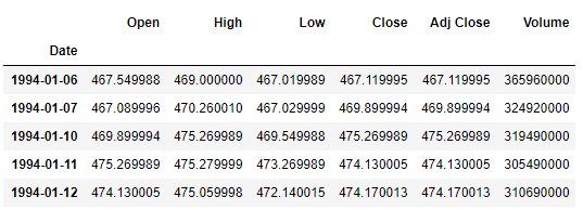
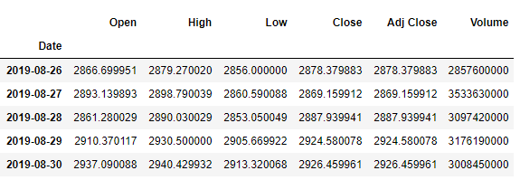
For this series of articles, the S&P 500 stock price from 1994–01–06 (6th January 1994) to 2019–08–30 (30th August 2019) is downloaded via the yfinance API.

In the above code cell, 2 standard libraries of python used in almost all data analysis projects: pandas and numpy are imported. Next to the plotting libraries of python: matplotlib.pyplot and seaborn are imported. The line sns.set() just applies a seaborn wrapper over all subsequent plots. Not including this line will have no effect on the outputs apart from some changes in styling.

Next, the yfinance library is imported. To download this, follow the instructions here. The download function of yfinance takes in the following arguments: tickers (a unique identifier for each time series at Yahoo Finance), interval (The time period between successive data points, which is 1 day or “1d” in this case), and, the start and end dates of the series. The data is then stored in a pandas dataframe (raw_data in this case).

The first few (shown using raw_data.head() ) and last few rows (shown using raw_data.tail() )of raw_data are as follows:

Extracting Relevant Series

In this series of articles, the Close prices of the S&P 500 market index are analyzed. Here, we extract the series we’re interested in:

Since the data is stock market data, we will not observe any value for the weekends. Thus, the time interval between 2 successive observations is 1 day even if the 2 observations are recorded on a Friday and then on a Monday. To convert our dates to follow the business days format (5 days a week), we use the asfreq() method of pandas with “b” as the argument.

Handling Missing Values

Next, let’s see whether this data has any missing values. This is an important preprocessing step, as the way we fill these values can have a huge impact on the tend.

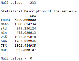
In the code cell above, data.spx.isnull().sum() takes the dataframe (data), extracts the column (spx) and applies the function isnull() to it. This results in a boolean array with True for every Null value encountered. The sum() function takes the sum of these boolean values. Since, True is represented as 1 and False as 0 , this gives the number of missing values in the spx series. The describe() function gives a few statistical measures of the series.

The number of null values (233) is clearly very small as compared to the count of observations (6459). Thus, a simple imputing function from pandas will be enough for this case. The fillna() function fills the missing values with the values encountered just before the missing value. This behavior is governed by the “ffill” (front fill) argument passed to the method argument. Click here for more information on other arguments for method.

Deriving S&P Returns and Volatility

Now that the data is cleaned, it can be used to build some other useful series that helps us to understand the market trends better. These are: Returns and Volatility.

Returns: The percent change in a stock price over a given amount of time. In this case, the returns over each day are calculated and stored in the column spx_ret.

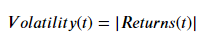
Volatility: The volatility in a market index refers to the fluctuations in its returns. To gauge the fluctuations or stability in the market, sometimes the magnitude of returns or squared returns are chosen. In this series, the magnitude of returns is chosen as the measure of volatility. The Volatility of spx is stored in the column spx_vol

Thus, Returns are a measure of the gain (positive returns) or loss (negative returns) of a market index, and Volatility (magnitude of Returns) is the measure of stability in the index.

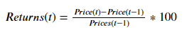
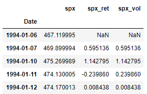
In the above code cell, the Returns and Volatility of spx is calculated. The pct_change() function takes the percent change in the current value and a previous value in the series. How far back should one go to take the previous value is controlled by the numeric value that is given as an argument to this function. Thus, the 1 argument in pct_change() takes the percent change between the current value and the value one-time step before. The mul() function is just used to scale the percents from 0–1to 0–100. Once the Returns are calculated, Volatility is calculated using the abs() function that retrieves the magnitude of the Returns.

Note: We’re calculating Returns, and subsequently Volatility, with respect to the data observed one time period previously. It means that for the first observation, we will not have any value (or Null/NA) for Returns and Volatility. This is obvious as for the first value (recorded on 1994–01–06 in this case), we do not have any previous value, and hence, we cannot calculate the Returns or the Volatility here.

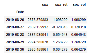
Let’s take a final look at our data by using the head() and the tail() functions to view the first and last 5 rows of the data, respectively.

Conclusion

In this article, the S&P 500 data is scrapped off the yfinance API, it is cleaned and used to derive other series like S&P 500 Returns and Volatility. In the next part, the 3 series generated will be visualized using common time series exploration techniques.

Links to other parts of this series

• Statistical Modeling of Time Series Data Part 1: Preprocessing
• Statistical Modeling of Time Series Data Part 2: Exploratory Data Analysis
• Statistical Modeling of Time Series Data Part 3: Forecasting Stationary Time Series using SARIMA
• Statistical Modeling of Time Series Data Part 4: Forecasting Volatility using GARCH
• Statistical Modeling of Time Series Data Part 5: ARMA+GARCH model for Time Series Forecasting.
• Statistical Modeling of Time Series Data Part 6: Forecasting Non – Stationary Time Series using ARMA

References

[1] 365DataScience Course on Time Series Analysis

[2] machinelearningmastery blogs on Time Series Analysis

---

Statistical Modeling of Time Series Data Part 1 : Data Preparation and Preprocessing was originally published in Towards AI on Medium, where people are continuing the conversation by highlighting and responding to this story.

Published via Towards AI