


Descriptive Statistics for Data Science: Explained
Last Updated on January 1, 2021 by Editorial Team
Author(s): Suhas V S
Data Science, Statistics
A detailed go through into various aspects of descriptive statistics using python.
It is often talked about that it is an essential requisite for a data scientist to have the ability to understand all types of data including the numerical and the categorical ones. This ability is stimulated by learning the different aspects of “Statistics”.
Statistics is mainly divided into 2 parts:
- Descriptive
- Inferential
Two important terminologies to be understood before moving any further are population and sample.
The population refers to the complete record of observation(rows) and features(columns). They are usually very big in size when solving real-time problems.
The sample is a part or subset of the population where statistical studies will be conducted on it to understand what it is going to be for the population it comes from.
From the understanding of population and sample, we will try to derive the definitions of descriptive and inferential statistics.
Descriptive Statistics – It is the study of the sample wherein we try to find out different measures(mean, median, variance…) and their dependence/inter-dependence on the existing features.
Inferential Statistics – After studying various measures and relationships in the sample, we try to generalize the measure to the whole population. It may be to estimate the mean of a certain numerical feature or to hypothesize a relationship between one or more features.
We can summarize that to make any kind of assumptions or estimations(inferential) about a large population, the understanding of its parameters and measures(descriptive) from its sample is very crucial. They may be divided into two different techniques but goes hand-in-hand to solve a real-time problem.
Descriptive Statistics:
1.Characteristics:
We will deal mostly with different measures that are important for us to develop a statistical acumen.
1.1 Measure of Central Tendency:
There are 3 measures of tendency namely mean, median, and mode. They are called so because each of the measures represents the data at its focal point which will allow us to make meaningful interpretations.
Mean:
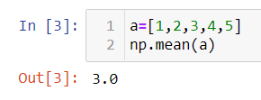
The mean is the average of the numerical values of a feature. When we have extreme values in the numerical list, the mean tends to move towards the extreme value. Hence, the mean is not recommended during such times. The way around in such times is to either go for a median value which we will see in the next block or we trim the extreme values on either side and then calculate the mean. Figure 1 shows the numpy function to calculate the mean.
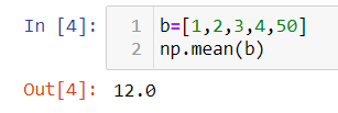
If we replace 5 with a more extreme value of 50, the mean changes from 3 to 12. Refer to Figure 2.
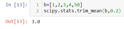
If we trim one value on either side of “b”, we will ignore the extreme values and take the mean for the rest of the data point. Refer to Figure 3 and see the variation of mean back to 3.
Note: Import numpy as np and scipy. stats to perform the above operations.
Median:
The median divides the datapoints into 2 equal halves and take the middle value as opposed to the average done in the case of mean. This makes the median immune to the presence of extreme values as it does not in any way use them for calculation.
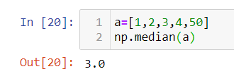
For example, refer to figure 4 where despite the presence of an extreme value of 50, we have been able to get the central tendency value(median) to be 3. This is the same output we have seen for the trimmed mean in figure 3.
Mode:
The mode is the frequency of the highest occurring element in the group. Refer to figure 5 where “3” is repeated with the highest count 2.

1.2 Measure of Location
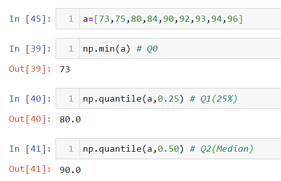
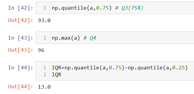
In this part, we will look into a measure called “quantile” which may or may not divide the numerical data into equal halves. If the data is divided into 4 different equal parts, then the quantiles become “quartiles” which is what we will be concentrating on here. Figure 6 is a pictorial representation of the quartiles using a “boxplot”.
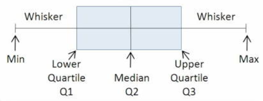
The above box plot has 5 important points:
a) Min(Q0): This is the lowest value in the numerical dataset.
b) Lower Quartile(Q1): This is the point that accounts for 25% of the data points.
c) Median(Q2): This point generally gives the idea about the 50% datapoint value of the dataset which divides the numerical data into 2 halves.
d) Upper Quartile(Q3): This is the point that accounts for 75% of the data points.
e) Max(Q4): This is the highest value in the numerical dataset.
The difference between Q3 and Q1 gives us information about the range of most of the values in the dataset. This difference is called the “Inter-Quartile Range(IQR)”.
Hence, IQR=Q3-Q1
Let us see how this concept can b realized in python with an example. Refer to figure 7 and 8 shown below.
1.3 Measures of Dispersion
This characteristic of the descriptive statistic gives an idea of the spread of the data. Meaning, it will tell us the deviation or distance of a data point concerning its mean. Many measures account for dispersion such as variance, standard deviation, and coefficient of variation. We will take each one up and study their features.
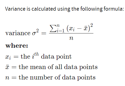
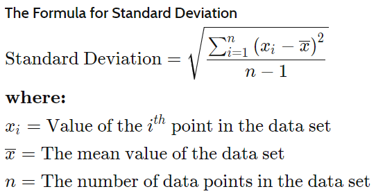
Variance:
The variance measures how far each number in the set is from the mean and hence from every other number in the set. Variance is depicted by the symbol: σ2(sigma squared). The formula is given by:
Standard Deviation(σ):
This measure also does the same job of letting us know how far the given data point is from the mean. It is by definition the square root of variance. If the data points are further from the mean, then there is a higher deviation within the data set. Hence, we can say the more spread out the data, the higher the standard deviation.
Coefficient of Variation:
This measure tracks the deviation of the data concerning its mean thereby giving an idea of where the data stands in terms of dispersion. It is the ratio of the standard deviation to its mean.
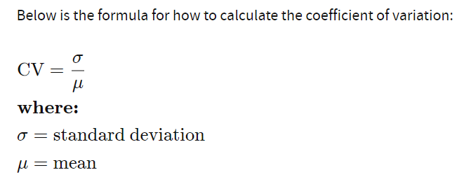
It is often used in “Stock Market Analysis” to determine the risk over the return where the “mean” is usually considered as the “return” and deviation as the “risk”. The higher the mean higher is the return and the same goes for the risk-standard deviation.
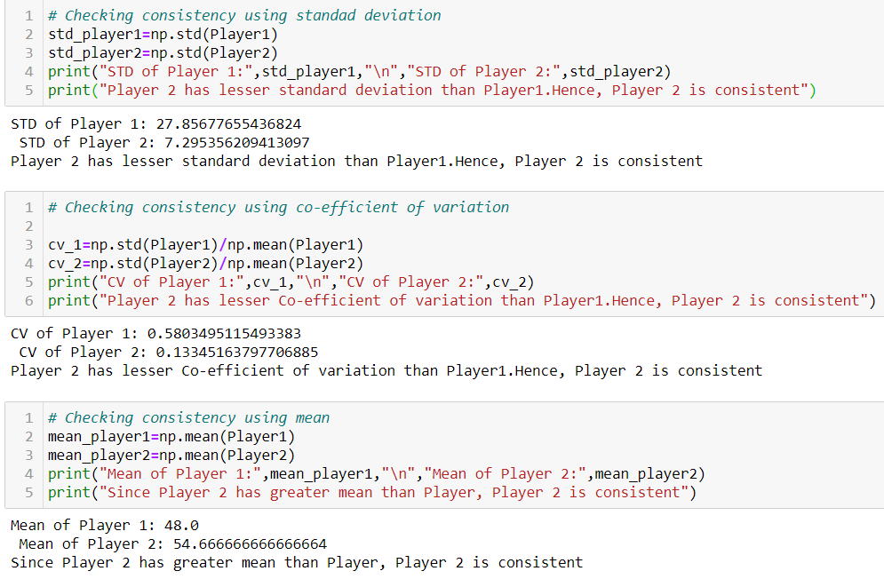
Example: Let us put our knowledge gained till now at work and find out which player is more consistent. Refer to figure 12.
Player1 = [100, 20, 30 ,40 ,50]
Player2 = [50,56,60,42,55,65]
Z-Score:
It also gives information about the spread of the data around the mean. Specifically, it is the distance of the data point from its mean to the standard deviation.
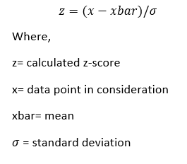
If z=0, it means that the data point is exactly equal to the mean value.
If z=1, it means that the data point is one standard deviation away from the mean.
Note: The function in python for z-score: scipy.stats.zscore()
1.4 Measures of Shape
When we are dealing with numerical data, it is important to understand the shape of the distribution which in turn is going to help in developing more accurate statistical acumen. There are two measures of shape namely skewness and kurtosis.
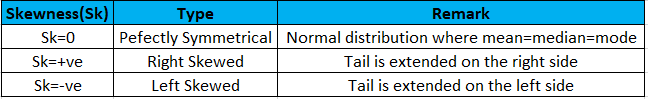
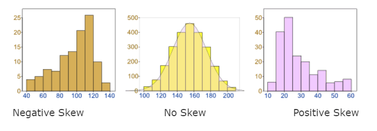
Skewness:
It is the degree of symmetry of the numerical data. If we plot a distribution on an x-y axis, skewness will let us know the direction and magnitude of the perturbation. More is the length of the tail on either side, more is the number of outliers or extreme values in the dataset.
The different types of skewness are given in the below table.
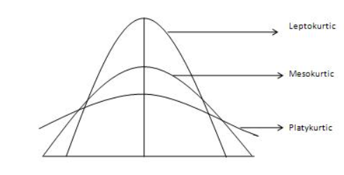
Kurtosis:
Similar to skewness, kurtosis tries to give information on the distribution plot considering the sharpness of the data. It also is used to find out how heavy is the tail of the distribution is.
Many of the statisticians say that kurtosis is the study of the peakedness of the data distribution. There are still some who feel that this definition is not completely true. One among them is Dr. Donald Wheeler and as per his understanding the definition goes like this, “The kurtosis parameter is a measure of the combined weight of the tails relative to the rest of the distribution.”
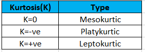
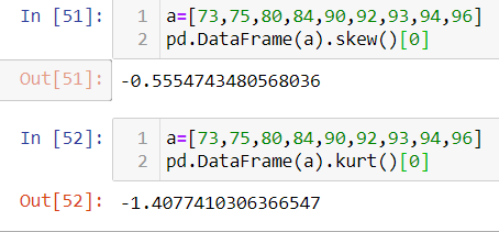
Note: We will have to import pandas package to use skew and kurt inbuilt functions. Let us an example. Here, for a list “a” the skewness and kurtosis values are negative.
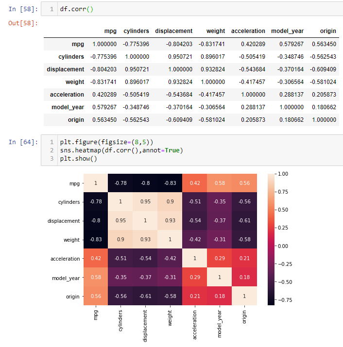
1.5 Covariance and Correlation
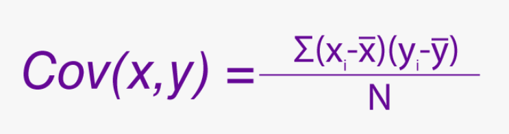
Variance is a measure that is used to find the spread of values in one numerical variable from its mean. To do it for 2 or more numerical variables, we use “covariance”. It ranges from -infinity to +infinity. It also tells whether two variables are related by measuring how the variables change with each other.
Since the range of covariance is from -infinity to +infinity, when the number of variables increases it becomes a harder task to compare and decide as the units and magnitude for different numerical variables will be different. Refer to Figure 21. To overcome this shortcoming, we will normalize the numerical values between -1 to +1 as opposed to -infinity to +infinity. Refer to figure 22.
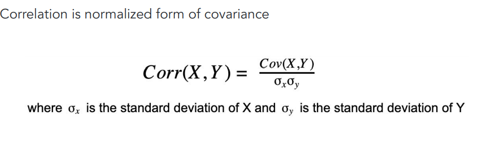
Note: corr=-1 means highly correlated in the negative direction. Same goes for corr=+1 which is highly correlated in the positive direction. Same can be deduced for the other -ve and +ve correlation values.
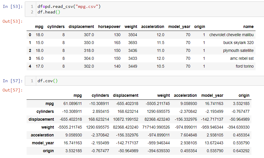
Getting covariance and correlation using pandas.
2.Probability and Bayes’ Theorem
When we are dealing with numbers and events, oftentimes we come across a question of the chance of an event happening when it is tried for “n” number of times. We would be needing to know the degree of uncertainty of an event happening. This is where the understanding of probability would give us meaningful insight.
By definition,

Example: Probability of ending up with value 3 on a dice(Only one trial)
Here, a we all know a dice has 6 faces and the number 3 can only come up once as it can not be repeated. Then, the probability of the event happening is 1/6.
Terminologies:
Sample space:
It is a space containing all the possible outcomes of an event happening for the “n” number of trials.
Sample Space size = (O)^n
where O= Number of uniquely exhaustive outcomes; n= number of trials.
Example: For a coin toss experiment done for 2 times.
Sample space size=(2)²=4 and sapce=[HH,HT,TH,TT]
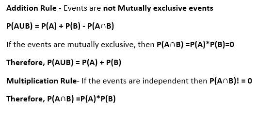
Mutually Exclusive Events: Two events A and B are said to be mutually exclusive if they cannot occur at the same time. Or the occurrence of A excludes the occurrence of B.
Example:When you toss a coin, getting a head or a tail are mutually exclusive as either head or tail will appear in case of an ideal scenario.
Independent Events: Two events A and B are said to be independent if the occurrence of A is in no way influenced by the occurrence of B. Likewise, the occurrence of B is in no way influenced by the occurrence of A.
Example:When you toss a fair coin and get head and then you toss it again and get a head.
Rules of Probability:
There are several rules when it comes to probability, but we will concentrate on the ones which we have seen in the above terminologies. Refer to figure 24.
Types of Probability:
- Marginal Probability: The term marginal is used to indicate that the probabilities are calculated using a contingency table (also called a joint probability table). The marginal probability of one variable (X) would be the sum of probabilities for the other variable (Y rows) on the margin of the table.
2. Joint Probability: Joint probability is the chance of a variable on X happening with another variable on the Y of the contingency table.
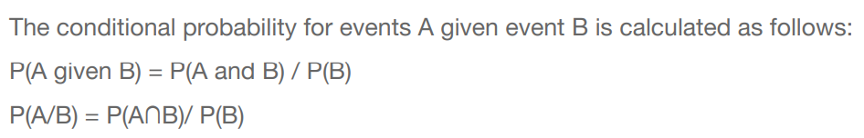
3. Conditional Probability: The probability of one variable on X happening given that another variable on the Y has already happened and vice-versa.
An Example to understand the probability types:
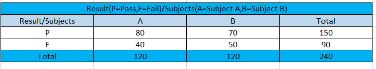
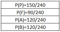
Figure 25 is a contingency table for students passing/failing in Subject A and Subject B.
The marginal probabilities are given by,
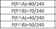
The joint probabilities are given by,
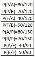
The conditional probabilities are given by,
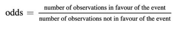
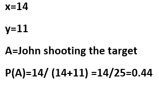
Odds:
The odds of an event is the ratio of the number of favorable events to the number of unfavorable events. It is another way of expressing probability. Here, we will have to derive the probability from the odds ratio.
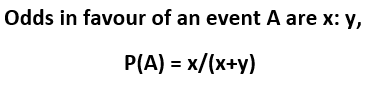
Example: The odds in favor of John shooting a target are 14:11. What is the probability of John shooting the target?
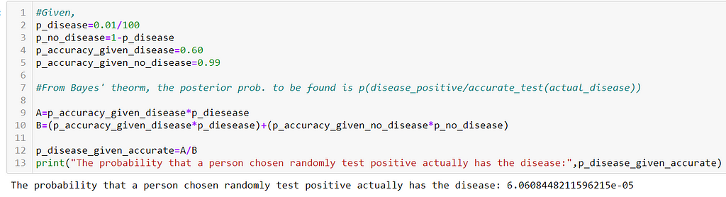
Bayes’ Theorem:
The Bayes’ theorem is an extension of the conditional probability wherein we will be calculating the posterior probability with the already known prior probability, the evidence, and the likelihood of the event happening.
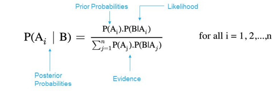
Example: A test for TB disease is 60% accurate when a person has the disease and 99% accurate when a person does not have the disease. If 0.01% of the population has TB disease, what is the probability that a person is chosen randomly from the population who test positive for the disease actually has the disease?
3. Probability Distributions
The probability distribution in simple terms is the distribution plot of the probability over the different outcomes of the event. We need to understand a very important term “Random Variable” before going any further as the entire concept of probability distributions is pivoted around it.
What is “Random Variable”?
In a random experiment, a variable takes different values as the result of the experiment and, that variable is called “Random Variable”. A random variable is discrete if it has a finite or countable number of possible outcomes that can be listed. A random variable is Continuous if it has an uncountable number of possible outcomes within a given interval. It is usually denoted by “X”.
Types of Probability distributions
Depending on the nature of the random variable whether it is discrete/continuous, we have 2 types of probability distributions.
- Discrete Probability Distribution
- Continuous Probability Distribution
Discrete Probability Distribution:
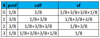
Probability Mass Function(PMF): The probability at discrete values of the random variable X is called “PMF”.
Cumulative Density Function(CDF) and Survival Function(SF) are the probability functions that add up individual pmfs cumulatively in opposite directions. The CDF adds it from left to right (includes the endpoint of the random variable). The SF adds the probabilities from right to left(excludes the final point).
Therefore, SF+CDF=1
Example: A coin is tossed 3 times. The random variable X= number of heads.
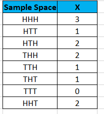
Let us realize the pmf, cdf, and sf.
We will discuss 2 types of discrete probability distributions namely Binomial and Poisson.
Binomial Distribution:
When do we use Binomial distribution?
a) When the number of trials of the experiment is “finite”.
b) When there only 2 unique outcomes.
c) The trials are independent.
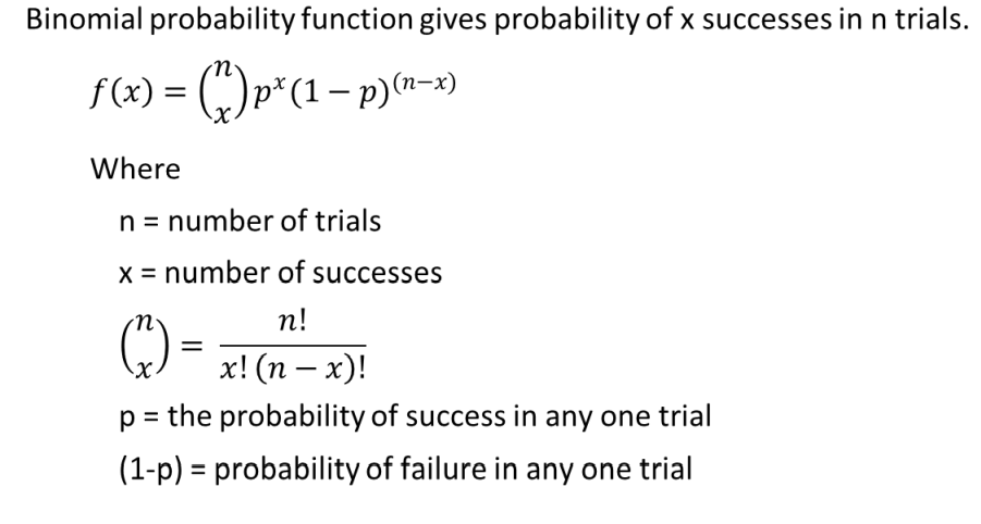
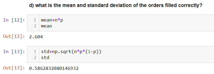
mean or expected value = n*p
variance=n*p*(1-p)
Let us see how we can realize binomial distribution in python using scipy.stats library.
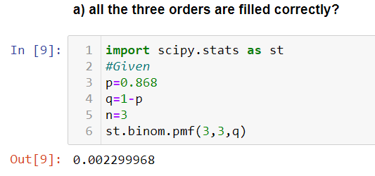
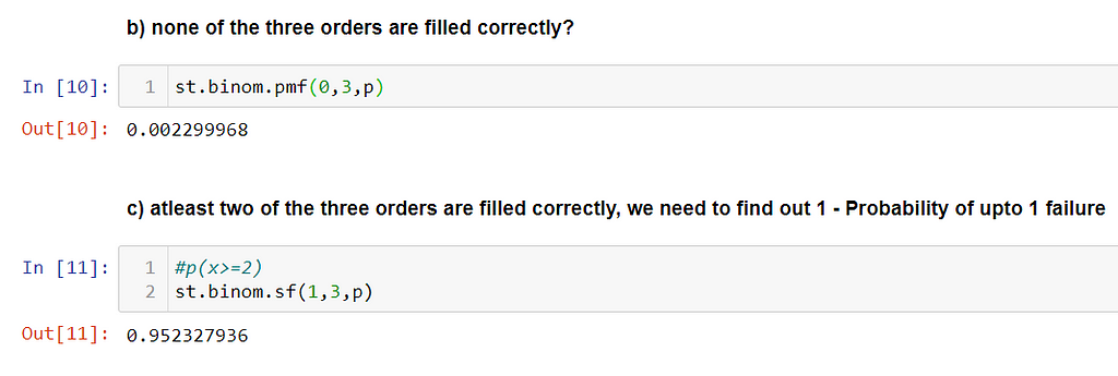
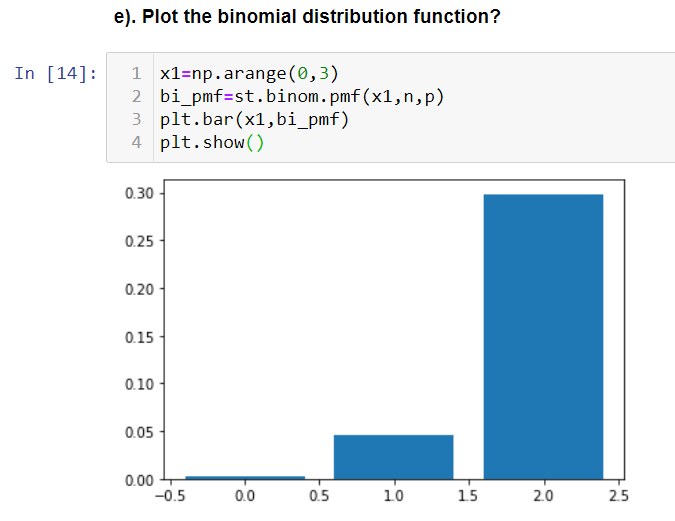
Problem: The percentage of orders filled correctly at Wendy’s was approximately 86.8%. Suppose that you go to the drive-through window at Wendy’s and place an order. Two friends of yours independently place orders at the drive-through window at the same Wendy’s.
What are the probabilities that,
a) all three orders are filled correctly?
b) none of the three are filled correctly?
c) at least two of the three orders will be filled correctly?
d) what is the mean and standard deviation of the orders filled correctly?
e) Plot the binomial distribution function
Since there are only 2 events orders filled correctly and not filled correctly and the number of trials is 3, we can use Binomial distribution.
It is a probability distribution used to estimate the number of occurrences over a specified period of time. When the number of trials approached “infinity”, the binomial probability nears “zero” hence we need a different technique to deal with. This is where we use “Poisson distribution”.
Let us see how we can realize Poisson distribution in python using scipy.stats library.
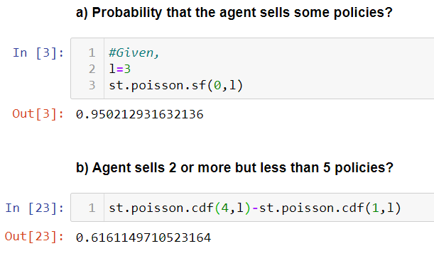
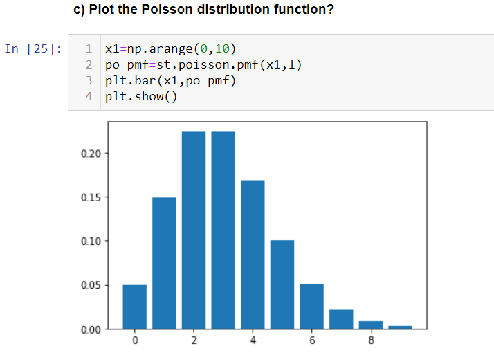
Problem: A Life Insurance agent sells on average 3 life insurance policies per week.
Use the Poisson law to calculate the probability that in a given week, he will sell
a) Some policies
b) 2 or more but less than 5 policies?
c) Plot the Poisson distribution function?
Continuous Probability Distribution:
As we know that for a continuous probability distribution, the random variable is continuous in nature. Below are the assumptions,
a. The probability at any point is 0. Hence, we make use of the area under the curve which is the probability.
b. We consider the probability over an interval of a random variable.
All the probability density functions cdf, sf works similarly to what we have seen in the discrete probability distributions.
We will understand the most important Normal distribution which is a continuous distribution.
Normal Distribution:
It deals with the gaussian or bell-shaped curve which maintains symmetry on either side of the curve where mean, median and mode are equal. The height and weight of the people, rainfall data, and most of the numerical data around us follow a normal distribution.
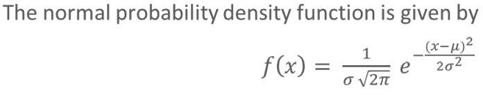
where, σ = standard deviation, u= population mean, e, and π are constants.
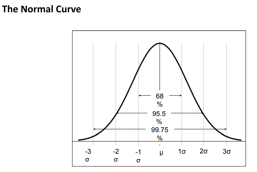
From Figure 47, we can say that 68% of the data points lie within -1σ and +1σ, 95.5% lie within -2σ and +2σ, and 99.75% lie within -3σ and +3σ.
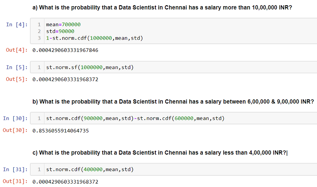
Let us see how we can realize Normal distribution in python using scipy.stats library.
Problem: The mean salaries of Data Scientists working in Chennai, India is calculated to be 7,00,000 INR with a standard deviation of 90,000 INR. The random variable salary of Data Scientists follows a normal distribution.
a) What is the probability that a Data Scientist in Chennai has a salary of more than 10,00,000 INR?
b) What is the probability that a Data Scientist in Chennai has a salary between 6,00,000 & 9,00,000 INR?
c) What is the probability that a Data Scientist in Chennai has a salary less than 4,00,000 INR?
This concludes the concepts and their realization using various python libraries in descriptive statistics. Having a strong understanding of these topics is very essential for handling complex problems that come in the inferential analysis. I have tried to include as many topics as possible which I thought would help. I will write on the inferential statistics as a continuation of this part. Till then, Happy reading!!!.
Descriptive Statistics for Data Science: Explained was originally published in Towards AI on Medium, where people are continuing the conversation by highlighting and responding to this story.
Published via Towards AI
Towards AI Academy
We Build Enterprise-Grade AI. We'll Teach You to Master It Too.
15 engineers. 100,000+ students. Towards AI Academy teaches what actually survives production.
Start free — no commitment:
→ 6-Day Agentic AI Engineering Email Guide — one practical lesson per day
→ Agents Architecture Cheatsheet — 3 years of architecture decisions in 6 pages
Our courses:
→ AI Engineering Certification — 90+ lessons from project selection to deployed product. The most comprehensive practical LLM course out there.
→ Agent Engineering Course — Hands on with production agent architectures, memory, routing, and eval frameworks — built from real enterprise engagements.
→ AI for Work — Understand, evaluate, and apply AI for complex work tasks.
Note: Article content contains the views of the contributing authors and not Towards AI.
Related posts


Recent Posts


")

