Titanic Survival Prediction — I

Last Updated on January 6, 2023 by Editorial Team

Author(s): Hira Akram

Data Analysis

Titanic Survival Prediction — I

Exploratory Data Analysis and Feature Engineering on the Titanic dataset

Titanic Kaggle competition is a great place to understand the machine learning pipeline. In this article, we will discuss the preliminary steps involved in building a predictive model. Let’s begin!

Competition Summary:

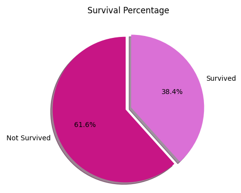
Our aim is to determine from a set of features whether a passenger would have survived the wreck. In other words, we will build a binary classification model that outputs ‘1’ stating that the passenger had survived the Titanic sinking and ‘0’ for not surviving.

Below is a visualization of the survival percentage in the provided training dataset. Based on this given percentage of ground truth; we will train five typical classification models and compare their performances:

Exploratory Data Analysis:

First and foremost step for building a machine learning model is EDA. This involves the following:

• Comprehend the underlying information like numbers of rows and columns, data types, look at a few samples from the data, general figures like mean median mode values.
• Indicate the proportion of missing values and decide how to address them.
• Data visualization.

So let’s explore the training set and establish an understanding of our data:

We gather the following information from the above code:

• Training data comprises a total of 891 examples and 12 features; including the ‘Survived’ flag.
• We have a mix of discrete and continuous features.
• There are three columns with missing values (Age, Cabin, Embarked)

Moving on, now let’s discuss each feature in detail to get a better intuition.

1. Pclass

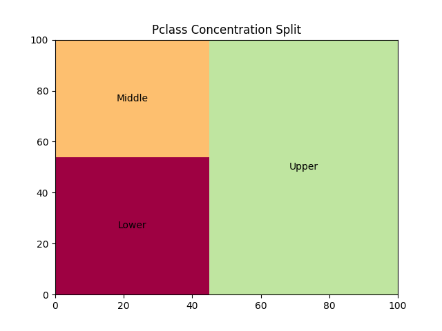
Our first feature to consider is Pclass. This is a categorical feature and it represents the socio-economic status of the passengers. We have plotted a treemap which clearly illustrates that the majority of the passengers belonged to the upper socio-economic status.

2. Name

Since the passenger names can not be used as is; therefore we have extracted the titles within the data to make more sense of this information.

3. Embarked

There were two missing values in this columns. We can either remove these rows or replace them with the mode value. Deleting rows would ultimately lead to date loss and given dataset is already very small; therefore we will go with option two. We also noticed that a high number of passengers embarked on Southampton.

4. Cabin

Although a huge number of values were missing from this column, but we extracted the alphabets specifying the cabin category. I will shortly discuss how we can make use of this to recreate features.

5. Age

Below code approximates the missing age values using IterativeImputer() function. Later on, we will utilize this column to build more complex features.

Feature Engineering

This method is used for adding complexity to the existing data; by constructing new features on top of the pre-existing columns. In order to better represent the underlying structure of the data; we can either split or merge information from different columns. This is one of the many techniques that can enhance our model performance altogether.

In the Titanic dataset we will include six additional columns using this method. Just like we carefully transformed all the passenger names into their titles; let’s look at some more columns.

Firstly, we will make use of the Parch and SibSp columns to count the number of family members that are on board, as below:

Moreover, an attribute like Fare per Family can also help understand the link between these two columns:

Ticket column in itself doesn’t seem quite useful, so we will construct a categorical column based on the nature of this data:

Concatenate the above-created column with the Cabin column that we transformed earlier, to gain some more value out of these features:

The following two features can also be built using the Age column. For ageBins, we will split the ages into four discrete equal-sized buckets using the pandas qcut() function.

Lastly, we will multiply Age with Fare to make a new numerical column.

Initially, the training dataset contained very simple features which were insufficient for the algorithm to search for patterns. Newly constructed features are designed to establish a correspondence between the dataset which ultimately enhances the model accuracy.

Now that our features are ready, we can move on to the next steps that are involved in data preparation.

Categorical Encoding

Since many algorithms can only interpret numerical data, therefore, encoding the categorical features is an essential step. There are three common workarounds for encoding such features:

1. One Hot Encoding (binary split)
2. Label Encoding (numerical assignment to each category)
3. Ordinal Encoding (ordered assignment to each category)

In our case, we will implement label encoding using sklearn LabelEncoder() function. We will label encode the below-mentioned list of columns that contain categorical information in form of words, alphabets or alphanumeric. This task can be achieved by using the following code:

['Pclass', 'Name', 'Sex', 'SibSp', 'Parch', 'Ticket', 'Fare', 'Embarked', 'familyMembers', 'ticketInfo', 'Cabin', 'Cabin_ticketInfo']

Standard Scaling

Continuous features can largely vary, resulting in very slow convergence hence impacting the model performance on the whole. The term scaling suggests, that we redistribute the feature values upon a fixed range so that the data dispersion is standardized. Once this is achieved, the model will efficiently converge to the global minima.

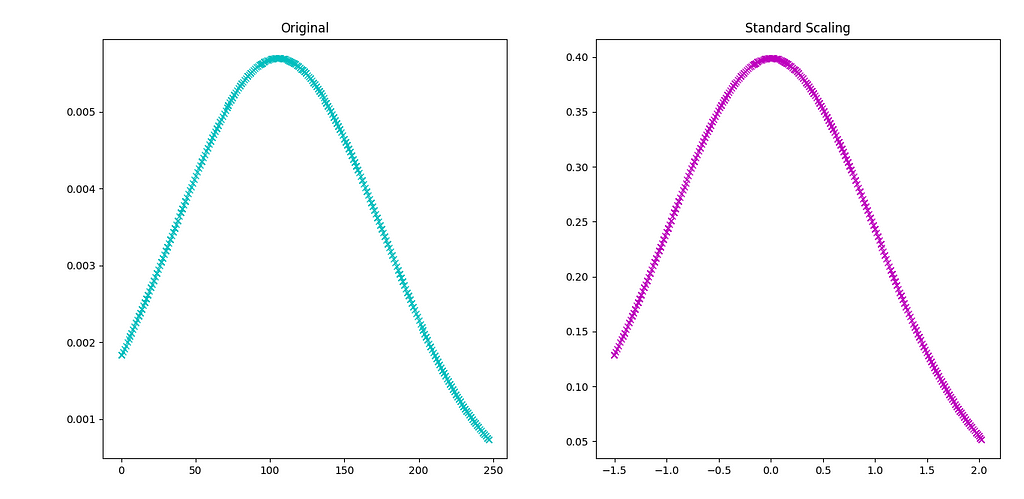
Originally, the Titanic data only had a single feature i.e. Fare which required scaling. While constructing new advanced features we included two more. Here’s how we’ll carry out standard scaling on all the continuous data:

Below is a comparison between unscaled and scaled ‘Fare’ values. We can see that new x range has approximately shrunk to ±2, also data is now distributed on zero mean:

Conclusion

Now that we feel confident about our data, let’s use it to train a bunch of models and pick the algorithm which suits best! In the next article, we will make survival predictions on the Titanic dataset using five binary classification algorithms.

Here are a few samples from the finalized training data:

---

Titanic Survival Prediction — I was originally published in Towards AI on Medium, where people are continuing the conversation by highlighting and responding to this story.

Published via Towards AI