Cracking the Code of Context: Word Vectorization Techniques in NLP

Author(s): Abhijith S Babu

Originally published on Towards AI.

You moved to a new town far from your country, where you happened to bump into someone in a coffee shop. A young woman around your age and instantly, you both were engaged in a conversation. It happened because both of you knew English. Just when you were thrilled to have met someone who spoke your language, the waiter came speaking in the native tongue, to take your order. Well, your new friend is ready to be a translator. As soon as you were back in your apartment, you rummaged through the internet, looking for courses to learn the native language. So it’s vivid that a common language is essential for proper communication between two entities.

In the buzzing domain of artificial intelligence, natural language processing is an exciting technology. It’s fascinating that a machine is able to understand what you are speaking in your native language. This facilitates a smooth mutual interaction between humans and computers. But shouldn’t there be a common language of communication for it to happen? As we know, humans speak a wide variety of languages, such as English, Spanish, French, Hindi, Mandarin, and so on. But the only language computers know is binary. Their entire world is built up of 0s and 1s.

If computers understand numbers and we understand languages such as English, there should be something that converts natural language to numbers. Word2vec comes to our rescue.

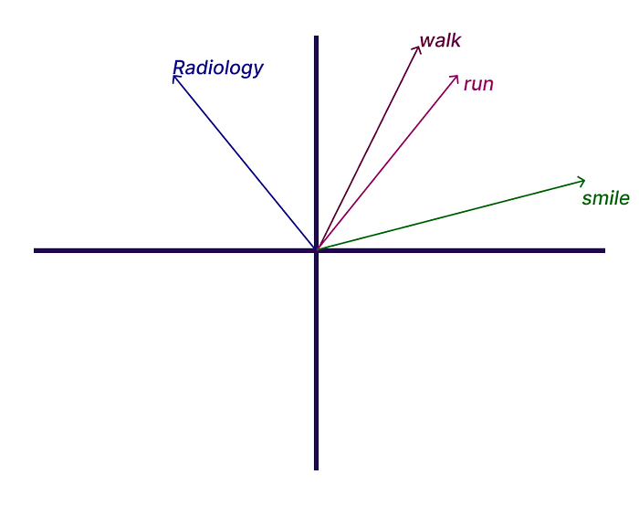
Word2vec represents the words in a sentence as a vector in a continuous space. The vectors capture the semantic relationship between the words in various contexts. Similar words have a similar vector. The figure below shows a 2D representation of such a vector space (the dimension of a vector space in actual NLP problems is way more than 2).

We can see similar words like walk and run close to each other. While smile and Radiology are unrelated words and are far apart. The words close to each other are called replaceable words, i.e., if you interchange those words in a sentence, the sentence will still make sense. The replaceability of two words can be calculated based on the cosine of the angle between the vectors of two words. This can take a value between -1 and 1, 1 meaning the words are strongly related. Some operations on the vectors can be used to perform tasks such as finding analogous words.

Word2vec is mainly used in word predictions. We might have seen features like autocomplete and autocorrect in our daily used apps like email. Word2vec is mainly used to predict the next word/words in an incomplete document or to fill in the missing words in a document. To perform these tasks, a machine learning model will be trained.

We can now see some ways in which natural languages are vectorized for real-life applications.

Here we are gonna train a spam filtering model using a relatively small dataset. For a proper model, we have to use a larger dataset. That will take a lot of time to run.

The data consists of several text messages which are either spam messages or not. It can be downloaded from here.

It is a text file in which each line has two fields, a label, and a sentence separated by a comma. The label is given spam for spam messages and ham for genuine messages.

I am going to implement this in Python. The program requires various libraries such as numpy, pandas, nltk, regex, gensim, and so on. If you don’t have them installed, you can install them using pip. I will show you all the packages imported for the program.

from gensim.models import Word2Vec
import numpy as np
from nltk.corpus import stopwords
import nltk
from nltk.corpus import stopwords
import pandas as pd
import string
import regex as re
from sklearn.feature_extraction.text import TfidfVectorizer
from sklearn.ensemble import RandomForestClassifier
from sklearn.metrics import precision_score,recall_score
from sklearn.model_selection import train_test_split
import gensim

Now that we have all the packages imported, we can start the implementation.

The first step is to clean and prepare the dataset.

messages = pd.read_csv("output.csv", delimiter="\t")
messages.columns = ["label", "text"]
 
 
def text_cleaner(text):
 nxt = "".join([char for char in text if char not in string.punctuation])
 nxt = re.split("\W+",nxt.lower())
 nxt = [k for k in nxt if k not in stopwords.words('english')]
 return nxt
 
messages["clean_text"] = messages['text'].apply(lambda x:text_cleaner(x))
print(messages.head())

I saved the dataset in a file called output.csv. I used pandas.read_csv() to read the file. The delimiter is set to “\t ”as the fields are separated in the dataset using tabs.

We gave titles to the two columns in the data as label and text.

Now we have to convert the text into tokens. Before that, we can clean the texts. First, we removed all the punctuation in the sentence. In Python, all the common punctuation's can be found in string.punctuation.

nxt = re.split(“\W+”,nxt.lower()) is used to split the sentence into a set of words using regex. I have also converted the words into lower-case since we don’t want our model to be case-sensitive.

Stopwords are those words which doesn’t contribute much to the gist of the sentence. There are around 170+ stopwords in English. They can be accessed from the nltk library using stopwords.words(‘english’). We can remove those words from our data to make our model light and efficient.

The data is now cleaned and tokenized and is stored in a new column called clean_text. The first 5 entries in the data can be printed using head() function.

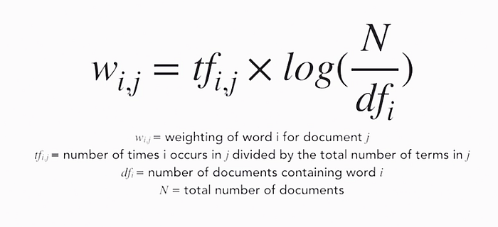
Now we have a set of tokens, which we have to convert into vectors before training. For that, let us use a property called TF-IDF (Term Frequency Inverse Document Frequency). The TF-IDF of a word in a document shows how important that word is to the document. It is directly related to the frequency of the word in the document and inversely related to the number of documents in the sample space. It can be calculated using

In Python, we can use a TfidfVectorizer class to create the vectors. To make the code simple, we are not creating a new column for cleaning and tokenizing. The text_cleaner function can be called in the TfidVectorizer().

new_vector = TfidfVectorizer(analyzer=text_cleaner)
x = new_vector.fit_transform(messages['text'])
x_features = pd.DataFrame(x.toarray())

x is now a 2D array in which each row represents a vector that contains the TF-IDF value of all the tokens in the sample space. If the word is not present in the sentence, the TF-IDF value of that token will be zero. Since this is the case for most of the words, we got a sparse matrix. The matrix is now converted to a pandas data-frame for training.

Here we are using the RandomForestClassifier provided by sklearn to train the model.

x_train, x_test, y_train, y_test = train_test_split(x_features,messages['label'],test_size=0.2)
rf = RandomForestClassifier()
rf_model = rf.fit(x_train,y_train)
y_pred = rf_model.predict(x_test)
precision = precision_score(y_test,y_pred,pos_label='spam')
recall = recall_score(y_test,y_pred,pos_label='spam')
print("precision = {} and recall = {}".format(round(precision,4),round(recall,4)))

The data is split into training and testing sets and the training set is passed to RandomForestClassifier to create a model. This model is tested with the test data and we got a precision of 1.0 and a recall of 0.8378. (you might get a slightly different value as I made some tweaks in the data I had).

Word2vec, on the other hand, works on a slightly different approach. It studies the word based on its position. This is done by analyzing the nearby words of a word. A window of a certain size is created around each occurrence of a word. In this way, the context of the usage of the word is learned. Let us see how it is done on the same dataset we used in the previous example.

The data is cleaned and tokenized and is stored in a new column as we did earlier. We can split that data into training and testing data and pass them into the word2vec model. Vectorization of the tokens is taken care of by the Word2Vec class found in the gensim package.

x_train, x_test, y_train, y_test = train_test_split(messages["clean_text"],messages["label"],test_size=0.2)
w2v_model = gensim.models.Word2Vec(x_train,vector_size=100,window=5,min_count=2)
w2v_model.save("mymodel.model")

The trained model can be saved to the local system so that we don’t have to train every time we run it.

Here we passed a minimum count of 2, which means that a vector is created only if there are at least 2 occurrences of the word in the whole data. Thus we can eliminate some words which don’t have any impact on the problem.

A word2vec model has a lot of in-built functionalities. For instance, if you want to find the words most similar to run in the model, you can use the most_similar() function.

mymodel = Word2Vec.load("mymodel.model")
similar_words = mymodel.wv.most_similar("run")
print(similar_words)

[('pls', 0.9978137612342834),
 ('yes', 0.9977635145187378),
 ('r', 0.9977442026138306),
 ('win', 0.9977269768714905),
 ('today', 0.9976850152015686),
 ('im', 0.9976809024810791),
 ('get', 0.9976732134819031),
 ('reply', 0.9976603984832764),
 ('new', 0.9976487159729004),
 ('one', 0.9976474046707153)]

The output we got is very crazy. That is because we used a small dataset for this training. Similar models trained on a large number of Wikipedia documents are available in gensim, which gives more accurate outputs.

Vectorizing natural language has a very large scope in machine learning. This technique can be applied in other domains as well. Sentimental analysis, text generation, and machine DNA classification are just a few of those applications. The success of word2vec played a key role in the development of these fields.

Join thousands of data leaders on the AI newsletter. Join over 80,000 subscribers and keep up to date with the latest developments in AI. From research to projects and ideas. If you are building an AI startup, an AI-related product, or a service, we invite you to consider becoming a sponsor.

Published via Towards AI