Automatic Differentiation with Python and C++ for Deep Learning

Author(s): Luiz doleron

Originally published on Towards AI.

This story explores automatic differentiation, a feature of modern Deep Learning frameworks that automatically calculates the parameter gradients during the training loop. The story introduces this technology in conjunction with practical examples using Python and C++.

Roadmap

• Automatic Differentiation: what is, the motivation, etc
• Automatic Differentiation in Python with TensorFlow
• Automatic Differentiation in C++ with Eigen
• Conclusion

Automatic Differentiation

Modern frameworks such as PyTorch or TensorFlow have an enhanced functionality called automatic differentiation [1], or, in short, autodiff. As its name suggests, autodiff automatically calculates the derivative of functions, reducing the responsibility of developers to implement those derivatives themselves.

What is the relevance of autodiff?

Every Deep Learning framework nowadays uses autodiff to compute the gradients of the trainable parameters.

Before autodiff became widely available, most of the time developing models was spent implementing code to calculate gradients (or actually debugging or removing bugs from the gradient code).

Therefore, autodiff was a game changer for deep learning popularization. It allowed even developers without solid calculus skills to implement complex machine-learning algorithms confidently. Even for developers with strong calculus knowledge, autodiff is helpful because it reduces the chance of a bug or suboptimal implementation.

Why does understanding autodiff matter?

In machine learning, autodiff completely abstracts the gradient calculation, usually providing exceptionally accurate and fast computations without any effort from the model developer. Usually. But not always.

Due to factors such as numeric instability, autodiff can fail in a few rare situations. Thus, understanding how autodiff works makes you ready to (i) use autodiff the most, (ii) detect when autodiff fails, and (iii) fix it when necessary.

It is also noteworthy that, in backpropagation, the calculation of gradients is the more critical and costly part, being completely accomplished by autodiff. Therefore, understanding autodiff becomes purely mandatory.

Automatic differentiation using TensorFlow

If you use Google TensorFlow, it’s possible you never thought of deriving a layer by yourself. Let us start with a simple example [2]:

import tensorflow as tf

class CustomLayer(tf.keras.layers.Layer):
 def __init__(self, num_outputs, activation):
 super(CustomLayer, self).__init__()
 self.num_outputs = num_outputs
 self.activation = activation

 def build(self, input_shape):
 self.kernel = self.add_weight("kernel",
 shape=[int(input_shape[-1]),
 self.num_outputs])

 def call(self, inputs):
 Z = tf.matmul(inputs, self.kernel)
 Y = self.activation(Z)
 return Y

This custom layer is basically a clone of tf.keras.layers.Densewith no bias. We can use it as follows:

def sin_activation(x):
 return tf.sin(x)

my_custom_layer = CustomLayer(2, sin_activation)

input = tf.constant([[-1., 0., 1.], [2., 3., 4.], [-1., -5., 2.]])

with tf.GradientTape() as tape:
 output = my_custom_layer(input)
 loss = tf.reduce_sum(output**2)

gradient = tape.gradient(loss, my_custom_layer.trainable_variables)
print("my_custom_layer.trainable_variables:\n", my_custom_layer.trainable_variables[0].numpy())
print("\ngradient:\n", gradient[0].numpy())

This code outputs something like:

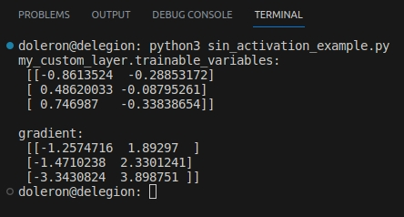
Since we are not using a built-in activation function (such as tf.keras.activation.relu), how does TensorFlow know how to calculate that gradient? The answer is simple: using automatic differentiation.

How autodiff works

Instead of asking the developer to provide an explicit derivative of sin_activation , TensorFlow computes the gradient using autodiff. But how does autodiff work?

May you have taken long calculus classes learning how to calculate derivatives of functions using the rules of differentiation. Is autodiff using those same rules to find the derivatives? Yes, but not in the same way you did.

The central idea [3] in autodiff is to break down the computation graph into elementary operations in which the derivatives are simple and known, then apply the chain rule recursively to compute the topmost derivative.

For instance, let us examine how the loss was computed in the last example:

This picture depicts the computation flow of the loss value. Using the chain rule, we can find the formula for the loss gradient with respect to weights:

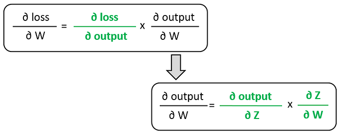
Which can be reduced to:

Note that those partial derivatives on the rightmost side are the leaf of the gradient computation graph. They are somehow elementary, which means that we cannot derive any other derivative from them.

Now, autodiff needs to find the value of these leaf gradients, which can be solved pretty straightforward by using basic calculus rules:

Finally, the gradient of loss with respect to the weights is found using the following computation:

Autodiff performs this graph computation under the wood without explicit interference from the developer. Great! So, what is the problem? The problem lies in the details!

Numerical instability comes into play

As said in the first part of this story, in some circumstances, autodiff fails due to the numerical instability of intermediary or leaf gradients. Consider the following example:

import tensorflow as tf

input = tf.Variable(100.0)

def function_using_autodiff(x):
 return 1./tf.exp(x)

with tf.GradientTape() as tape:
 output = function_using_autodiff(input)
gradient = tape.gradient(output, input)

print("output using autodiff: ", output.numpy())
print("gradient using autodiff: ", gradient.numpy())

This program outputs:

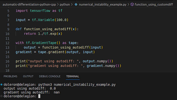
In this case, although the function was correctly evaluated at x=100, the gradient provided by autodiff was nan. Let us solve this problem by using a custom gradient. First, let us check the function expression:

The derivative of this function is:

Now, we can implement this derivative as a custom gradient [4] as follows:

import tensorflow as tf

@tf.custom_gradient
def function_using_customdiff(x):
 e = tf.exp(x)
 def grad(upstream):
 return upstream * -tf.exp(-x)
 return 1./tf.exp(x), grad

with tf.GradientTape() as tape:
 output = function_using_customdiff(input)
gradient = tape.gradient(output, input)

print("output using custom diff: ", output.numpy())
print("gradient using custom diff: ", gradient.numpy())

This time, the gradient is correctly evaluated:

Sometimes, the numerical instability comes from a theoretical property of the function at hand. For example, the derivative of the following function:

is

which is clearly undefined when x = 0, even though f(0) = 0! We can also use a custom gradient to provide a convenient (engineering) solution for cases like this.

Now that we understand how to use autodiff in Python/TensorFlow, let us learn how to use this technology in C++ programs with Eigen.

Autodiff in C++ with Eigen

Eigen is one of the most well-succeeded high-performing algebra libraries for C++ ever. If you are unfamiliar with Eigen, I recommend reading one of my previous stories on Medium.

Using Eigen Autodiff [5] is pretty straightforward. Let us start with a simple — but illustrative — example. Consider the following function:

template<typename T>
T my_function(const T& x)
{
 T result = T(1)/(T(1) + exp(-x));
 return result;
}

Note that we are defining this function as a template function. Without going into the details, a template function is a mold for a function. Not a function, really. Templates like this are useful because we can reuse my_functionwith different data types.

Usually, we would call our functions using types like float, double, or int. However, to make Eigen Autodiff work, we have to pass values as Eigen::AutoDiffScalar. Check the example below:

#include <iostream>
#include <unsupported/Eigen/AutoDiff>

int main(int, char **)
{

 Eigen::AutoDiffScalar<Eigen::VectorXd> X;

 X.derivatives() = Eigen::VectorXd::Unit(1, 0);
 X.value() = 2.f;

 auto Y = my_function(X);

 std::cout << "Y: " << Y << "\n\n";
 std::cout << "derivatives:\n" << Y.derivatives() << "\n";

 return 0;
}

The first point here is the header unsupported/Eigen/AutoDiff. In this file, Eigen defines the type Eigen::AutoDiffScalar used to type the variable X. Check again the following two lines:

X.derivatives() = Eigen::VectorXd::Unit(1, 0);
X.value() = 2.f;

These lines set the value of X and its index. Since X is the only variable in this example, its index is 0.

Now, we can pass X to my_function as usual:

auto Y = my_function(X);

Y is a Eigen::AutoDiffScalar as well. As we can see in the code, the value of each partial derivative of Yis stored in the derivatives() array. Running this code results in the following output:

Y stores both the function output value and the derivative with respect to X. How can we know if these values are correct? You may be noted that my_function is indeed the sigmoid formula:

The sigmoid derivative formula is well-known as:

Thus, a simple calculator can double-check the values of σ(2) = 0.8808 and σ’(2) = 0.10499.

This was — intentionally — a very simple example. Let us try something a bit more challenging now.

Implementing the CustomLayer using C++ and Eigen

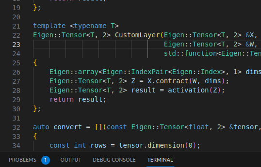
Once we know how to use autodiff in C++ with Eigen, we can finally rewrite the CustomLayer example, this time using C++:

#include <unsupported/Eigen/CXX11/Tensor>

template <typename T>
Eigen::Tensor<T, 2> CustomLayer(Eigen::Tensor<T, 2> &X, Eigen::Tensor<T, 2> &W, std::function<Eigen::Tensor<T, 2>(Eigen::Tensor<T, 2>&)> activation)
{
 Eigen::array<Eigen::IndexPair<Eigen::Index>, 1> dims = { Eigen::IndexPair<Eigen::Index>(1, 0) };
 Eigen::Tensor<T, 2> Z = X.contract(W, dims);
 Eigen::Tensor<T, 2> result = activation(Z);
 return result;
};

Here, it urges to highlight three points:

• We are using Eigen tensors instead of Eigen matrices. If you are unfamiliar with Tensors in Eigen, read this story;
• We are performing a contraction. Contractions are the multidimensional generalization of the matrix product.
• We are using a template function. A template class would also work. The point here is to define it as a template like we did in the previous example.

Furthermore, we are passing the activation as a std::function. Let us define it now:

template <typename T>
T sine(T t) {
 return sin(t);
}

template <typename T>
Eigen::Tensor<T, 2> sin_activation(Eigen::Tensor<T, 2> & P) {
 Eigen::Tensor<T, 2> result = P.unaryExpr(std::ref(sine<T>));
 return result;
};

Again, we are using templates. Everything here is straightforward. We are simply using unaryExpr to map P using the sin(t) function. Now, we can finally invoke CustomLayer:

#include <unsupported/Eigen/AutoDiff>

typedef typename Eigen::AutoDiffScalar<Eigen::VectorXf> AutoDiff_T;

int main(int, char **)
{

 Eigen::Tensor<float, 2> x_in(3, 3);
 x_in.setValues({{-1., 0., 1.}, {2., 3., 4.}, {-1., -5., 2.}});

 Eigen::Tensor<float, 2> w_in(3, 2);
 w_in.setRandom();

 Eigen::Tensor<AutoDiff_T, 2> X = convert(x_in);
 Eigen::Tensor<AutoDiff_T, 2> W = convert(w_in, 0, w_in.size());

 auto Y = CustomLayer(X, W, sin_activation<AutoDiff_T>);

 auto output = Y * Y;
 auto LOSS = ((Eigen::Tensor<AutoDiff_T, 0>)output.sum())(0);

 auto dY_dW = gradients(LOSS, W);

 std::cout << "trainable_variables:\n" << W << "\n\n";
 std::cout << "gradient:\n" << dY_dW << "\n\n";
 std::cout << "output:\n" << output << "\n\n";
 std::cout << "loss:\n" << LOSS << "\n\n";

 return 0;
}

As its name suggests, the function convert converts the original canonical tensors x_in and w_in into Eigen::Tensor<AutoDiff_T, 2> tensors. As we discussed in the last example, the Eigen::AutoDiffScalar type is mandatory for Eigen autodiff to work. convert is defined as follows:

auto convert = [](const Eigen::Tensor<float, 2> &tensor, int offset = 0, int size = 0)
{
 const int rows = tensor.dimension(0);
 const int cols = tensor.dimension(1);

 Eigen::Tensor<AutoDiff_T, 2> result(rows, cols);

 for (int i = 0; i < rows; ++i)
 {
 for (int j = 0; j < cols; ++j)
 {
 int index = i * cols + j;
 result(i, j).value() = tensor(i, j);
 if (size) {
 result(i, j).derivatives() = Eigen::VectorXf::Unit(size, offset + index);
 }
 }
 }

 return result;
};

Note the two lines when we invoke convert:

Eigen::Tensor<AutoDiff_T, 2> X = convert(x_in);
Eigen::Tensor<AutoDiff_T, 2> W = convert(w_in, 0, w_in.size());

It turns out that we are looking only for the partial derivatives of W. The next section explains how to calculate the partial derivatives with respect to X as well.

In the and, Y has the layer output value and the partial derivatives with respect to W. Then, one can use a function gradients to unpack the gradients:

auto gradients(const AutoDiff_T &LOSS, const Eigen::Tensor<AutoDiff_T, 2> &W)
{

 auto derivatives = LOSS.derivatives();

 int index = 0;

 Eigen::Tensor<float, 2> result(W.dimension(0), W.dimension(1));
 for (int i = 0; i < W.dimension(0); ++i)
 {
 for (int j = 0; j < W.dimension(1); ++j)
 {
 float val = derivatives[index];
 result(i, j) = val;
 index++;
 }
 }

 return result;
}

After building and running it, this code outputs something like this:

As expected, a similar output to the one generated by the Python/TensorFlow example.

Obtaining the derivatives with respect to X

In the last example, we computed only the gradient of W. If we were also interested in computing the partial derivatives of X, we must implement the following changes:

int size = x_in.size() + w_in.size();
Eigen::Tensor<AutoDiff_T, 2> X = convert(x_in, 0, size);
Eigen::Tensor<AutoDiff_T, 2> W = convert(w_in, x_in.size(), size);

This code basically notifies Eigen to keep tracking the derivative of X as well. Note that, to unpack both Xand W, you have to change the gradients function as well:

auto gradients(const AutoDiff_T &Y, const Eigen::Tensor<AutoDiff_T, 2> &X, const Eigen::Tensor<AutoDiff_T, 2> &K)
{

 auto derivatives = Y.derivatives();

 int index = 0;
 Eigen::Tensor<float, 2> dY_dX(X.dimension(0), X.dimension(1));
 for (int i = 0; i < X.dimension(0); ++i)
 {
 for (int j = 0; j < X.dimension(1); ++j)
 {
 float val = derivatives[index];
 dY_dX(i, j) = val;
 index++;
 }
 }

 Eigen::Tensor<float, 2> dY_dK(K.dimension(0), K.dimension(1));
 for (int i = 0; i < K.dimension(0); ++i)
 {
 for (int j = 0; j < K.dimension(1); ++j)
 {
 float val = derivatives[index];
 dY_dK(i, j) = val;
 index++;
 }
 }

 return std::make_pair(dY_dX, dY_dK);
}

Now, you should call gradients accordingly:

auto [dY_dX, dY_dW] = gradients(LOSS, X, W);

Passing either X and W. After these changes, running the program again results in the following output:

Alternatives to autodiff

The way we calculated the fourier_activation gradient “by hand” at the beginning of this story is known as symbolic differentiation.

In symbolic differentiation, a program function needs to be converted to an abstract mathematical expression. The expression is then differentiated using calculus rules to obtain a derivative form. Finally, the derivative form is used to get an output. A program to implement this process is not often efficient. Despite the efforts of highly competent people working on this subject, I’m afraid to say that symbolic differentiation (only) is not suitable for general software applications.

Another alternative to autodiff is numeric differentiation. In numeric differentiation, the derivative is calculated by an interactive (discrete) process. In numeric differentiation, the derivative is approximated by a finite number of steps. A difficulty with numeric differentiation is that this process introduces rounding errors due to inevitable discretization. Furthermore, very often, numeric differentiation is slower than autodiff.

Conclusion

This story introduced autodiff, one of the most cutting-edge subjects in the field of deep learning. The success of implementing this technology in open-source packages has been an enormous achievement in the development and popularization of artificial intelligence for the last two decades.

Particularly, it amazes me how simple and concise Eigen Autodiff is. Unfortunately, there is not much documentation about it. If these examples are not suitable to your use case, I recommend checking for more examples in the Eigen repository on GitLab.

References

[1] Baydin et al., Automatic Differentiation in Machine Learning: a Survey, Journal of Machine Learning Research 18 (2018) 1–43

[2] TensorFlow documentation, Custom layers

[3] Roger Grosse, CSC321 Lecture 10: Automatic Differentiation, CS at Toronto University

[4] TensorFlow documentation, Advanced automatic differentiation

[5] Patrick Peltzer, Johannes Lotz, Uwe Naumann, Eigen-AD: Algorithmic Differentiation of the Eigen Library, ICCS 2020: 20th International Conference

Join thousands of data leaders on the AI newsletter. Join over 80,000 subscribers and keep up to date with the latest developments in AI. From research to projects and ideas. If you are building an AI startup, an AI-related product, or a service, we invite you to consider becoming a sponsor.

Published via Towards AI