Analyzing MRI Scans With AI (Tensorflow) Is Easier Than You Think

Author(s): Laszlo Fazekas

Originally published on Towards AI.

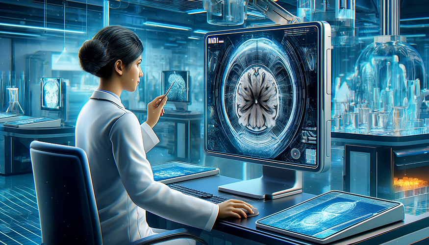
A few weeks ago, I had an MRI scan. That’s when it occurred to me to wonder how complicated it would be to evaluate MRI images with the help of AI. I had always thought that this was a complex problem that only universities and research institutes dealt with. Eventually, I had to realize that it’s actually not that difficult a task, and in fact, there are simple, well-proven methods for this.

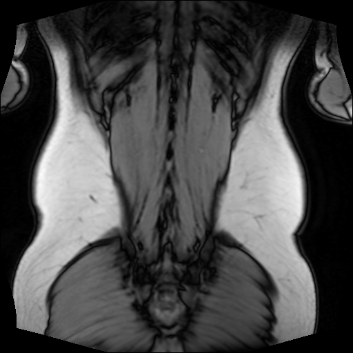
Obviously, the first question is how to read MRI scans with Python. Fortunately, most MRI devices produce data in DICOM format, from which grayscale images can be exported easily. I received my MRI scans on a CD. With the help of ChatGPT, it took just a quarter of an hour to put together a small script that exports the images.

The code expects two parameters. The first is the path to the DICOMDIR file, and the second is a directory where the images will be saved in PNG format.

To read the DICOM files, we use the Pydicom library. The structure is loaded using the pydicom.dcmread function, from which metadata (such as the patient’s name) and studies containing the images can be extracted. The image data can also be read with dcmread. The raw data are accessible through the pixelarray field, which the save_image function converts to PNG.

The following 512×512 image, for example, depicts my back, which is exported by the above script:

Now that we know how easy it is to access MRI scans, let’s see how complicated it is to process them.

After a quick search, I found an MRI dataset on Kaggle that contains brain MRI scans categorized by tumor type: three groups according to the type of tumor, and a fourth group that includes scans of healthy brains. I also found a notebook with a neural network that can categorize the images with perfect accuracy. I expected a complex architecture, but to my surprise, it was not complicated at all. It was a standard convolutional network that was able to recognize the tumors so effectively.

One of the first neural network architectures I encountered was the Tensorflow CNN example, which categorizes images from the well-known CIFAR-10 dataset. The CIFAR-10 dataset contains 60,000 images categorized into ten classes, such as dogs, cats, and the like. The structure of the sample CNN is as follows:

model = models.Sequential()
model.add(layers.Conv2D(32, (3, 3), activation='relu', 
 input_shape=(32, 32, 3)))
model.add(layers.MaxPooling2D((2, 2)))
model.add(layers.Conv2D(64, (3, 3), activation='relu'))
model.add(layers.MaxPooling2D((2, 2)))
model.add(layers.Conv2D(64, (3, 3), activation='relu'))
model.add(layers.Flatten())
model.add(layers.Dense(64, activation='relu'))
model.add(layers.Dense(10))

As you can see, the network architecture is quite simple. At the beginning of the network, convolutional and max pooling layers alternate to extract important features. This is followed by 2 dense layers, which classify the images into 10 categories based on the features. It’s not a very complex network, yet it is quite effective at recognizing the images in the CIFAR-10 dataset. (Those interested in a deeper understanding of how the network works can read more in the official TensorFlow tutorial.)

After this, let’s look at the structure of the network that recognizes tumors:

model = Sequential([
 # Input tensor shape
 Input(shape=image_shape),
 
 # Convolutional layer 1
 Conv2D(64, (5, 5), activation="relu"),
 MaxPooling2D(pool_size=(3, 3)),

 # Convolutional layer 2
 Conv2D(64, (5, 5), activation="relu"),
 MaxPooling2D(pool_size=(3, 3)),

 # Convolutional layer 3
 Conv2D(128, (4, 4), activation="relu"),
 MaxPooling2D(pool_size=(2, 2)),

 # Convolutional layer 4
 Conv2D(128, (4, 4), activation="relu"),
 MaxPooling2D(pool_size=(2, 2)),
 Flatten(),

 # Dense layers 
 Dense(512, activation="relu"),
 Dense(num_classes, activation="softmax")
])

It is very similar. Here, instead of three, there are four convolutional layers with larger kernel sizes and more channels, and the dense layer contains 512 neurons instead of 64. This network only differs in the number of parameters from the one we used to recognize cats and dogs. Nevertheless, this network can recognize tumors in MRI images with 99.7% accuracy. Anyone can clone the notebook on Kaggle and try out the network themselves.

I just want to point out how simple it can be to extract and process medical data in certain cases and how problems that seem complex, like detecting brain tumors, can often be quite effectively addressed with simple, traditional solutions.

Therefore, I would encourage everyone not to shy away from medical data. As you can see, we are dealing with relatively simple formats, and using relatively simple, well-established technologies (convolutional networks, vision transformers, etc.), a significant impact can be achieved here. If you join an open-source healthcare project in your spare time just as a hobby and can make even a slight improvement to the neural network used, you could potentially save lives!

Join thousands of data leaders on the AI newsletter. Join over 80,000 subscribers and keep up to date with the latest developments in AI. From research to projects and ideas. If you are building an AI startup, an AI-related product, or a service, we invite you to consider becoming a sponsor.

Published via Towards AI