Exploration of Joint PMFs: Their Applications in Data Science (Part 1)

Author(s): Ghadah AlHabib

Originally published on Towards AI.

Introduction to Joint PMFs

When dealing with discrete random variables, the joint probability mass function (PMF) is a fundamental concept in probability theory and statistics. Understanding it is crucial for analyzing the relationships between different random variables and for performing multivariate probability calculations. For instance, if you have two discrete random variables, X and Y, the joint PMF gives you the probability that Y takes on a specific value x and Y takes on a specific value y simultaneously.

Why are joint PMFs of multiple random variables important in data science?

Joint PMFs help to understand how different variables interact with each other and identify patterns and correlations by providing the probabilities of combinations of variable outcomes.

They are useful for testing the independence of variables. By comparing the joint PMF to the product of the marginal PMFs, we can determine if the variables are independent. If the joint PMF equals the product of the marginal PMFs for all values, the variables are considered independent, which simplifies further analysis.

Furthermore, multivariate distributions leverage joint PMFs to model the behavior of several random variables simultaneously and analyze scenarios where outcomes are influenced by multiple variables. In Bayesian statistics, joint PMFs are crucial for computing posterior probabilities and updating the probability of hypotheses based on the observed data.

What is a Joint Probability table?

A joint probability distribution represents a probability distribution for two or more random variables. The joint probability table is a representation of the joint probability mass function (PMF) for discrete random variables and it’s a function that gives the probability that each possible pair of outcomes occurs.

A joint probability table contains the following elements:

1. Header Rows and Columns: These indicate the possible values or categories of each random variable.
2. Cell Probabilities: Each cell in the table corresponds to the joint probability of the respective values of X and Y.
3. Marginal Probabilities: Often, the rightmost column and the bottom row are added to show the marginal probabilities for X and Y respectively, which are computed by summing the joint probabilities across rows for X and down columns for Y.
4. Total Probability: The bottom right corner of the table (if marginal probabilities are included) should show the total probability, which must be 1, as it sums all joint probabilities.

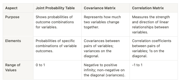
How is a Joint Probability Table Different from a Covariance Matrix and Correlation Matrix?

Use Case 1: Analyzing the Behavior of Customers in Purchasing Different Products

This can be achieved by analyzing the joint probability of customers buying multiple products together. Why should we do this analysis? To aid in achieving cross-selling and upselling as well as strategic pricing decisions. So, by understanding which products are frequently bought together, retailers can design targeted strategies. For example, if data shows a high joint probability of customers buying shampoo and conditioner together, placing these items near each other can increase sales. In another example, if two products are often purchased together, a discount on one might drive sales of the other, even if the second item is not discounted.

Let’s start with something simple and then we’ll build the concepts along the way:

import numpy as np
import pandas as pd


data = np.array([
 [1, 1],
 [0, 1],
 [1, 0],
 [1, 1],
 [0, 0],
 [1, 0],
 [0, 1],
 [1, 1],
 [1, 1],
 [0, 1],
 [1, 0],
 [1, 1],
 [0, 0],
 [1, 0],
 [0, 1],
 [1, 1],
 [1, 1],
 [0, 1],
])

df = pd.DataFrame(data, columns=['Product A', 'Product B'])

# P(A=0, B=0), P(A=0, B=1), P(A=1, B=0), P(A=1, B=1)
joint_probabilities = df.groupby(['Product A', 'Product B'])
 .size().div(len(df)).unstack(fill_value=0)

df_joint_pmf = pd.DataFrame({
 "Product B (Yes)": [joint_probabilities[1][1], 
 joint_probabilities[1][0], 
 joint_probabilities[1][1] + joint_probabilities[1][0]],
 "Product B (No)": [joint_probabilities[0][1], 
 joint_probabilities[0][0], 
 joint_probabilities[0][1] + joint_probabilities[0][0]],
 "Total": [joint_probabilities[1][1] + joint_probabilities[1][0], 
 joint_probabilities[0][1] + joint_probabilities[0][0], 1]
}, index=["Product A (Yes)", "Product A (No)", "Total"])

In this code snippet, we will generate synthetic data to mimic a real dataset where each row is a customer, and the columns represent two products. The first column is the first product, and the second column is the second product, where 1 indicates that a product is bought and 0 was not.

The joint probabilities are calculated for different combinations of purchasing behaviors for ‘Product A’ and ‘Product B’. This is done by grouping the data by the values of ‘Product A’ and ‘Product B’, counting the occurrences of each combination, and then dividing by the total number of observations to get the probabilities.

If any combination of product purchases is not present in the dataset (for example, if there are no customers who didn’t buy both products together), the unstack method with fill_value=0 ensures that the missing combination is present in the table with a probability of 0.

Moving on to an example with a real dataset:

Here we will use a dataset from an online retail store to analyze the behavior of customers in purchasing different products.

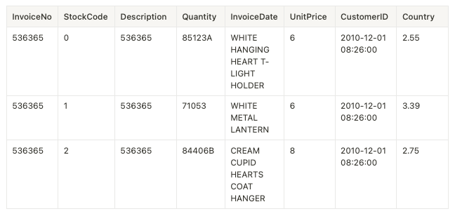
These are the first 5 rows of the dataset. Each row is a log of a particular product ordered (not an order with one or more products)

import pandas as pd

df = pd.read_excel('Online Retail.xlsx')

df = df[~df['InvoiceNo'].astype(str).str.contains('C')]
df = df.dropna(subset=['CustomerID'])

df['Category'] = df['StockCode'].astype(str).str[0]
df['Purchased'] = 1 

pivot_df = df.pivot_table(index='InvoiceNo', columns='Category', 
 values='Purchased', fill_value=0, aggfunc='max')

categories = ['2','4']
pivot_df = pivot_df[categories]


joint_probabilities = pivot_df.groupby(categories).size().div(len(pivot_df))

df_joint_pmf = pd.DataFrame({
 "Category 4 (Yes)": [joint_probabilities[1][1], 
 joint_probabilities[1][0],
 joint_probabilities[1][1] + joint_probabilities[1][0]],
 "Category 4 (No)": [joint_probabilities[0][1], 
 joint_probabilities[0][0], 
 joint_probabilities[0][1] + joint_probabilities[0][0]],
 "Total": [joint_probabilities[1][1] + joint_probabilities[0][1], 
 joint_probabilities[1][0] + joint_probabilities[0][0], 1]
}, index=["Category 2 (Yes)", "Category 2 (No)", "Total"])

We will first clean the dataset to remove all canceled orders and missing customer IDs and then create a new column indicating the category of the product ordered. This category is obtained from the ‘StockCode’ column and is just a simple strategy to create the category of the order for the sake of demonstration.

Afterward, we will add a marker to indicate purchase and aggregate the data to see which categories were bought together. So, we’ll use pivote_table to create the following dataframe, indexed it by the ‘InvoiceNo’, and make the columns of the table to be the categories of the products.

The pivot table will look like the following:

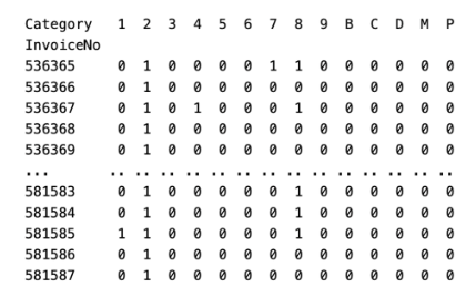
We will use the aggfunc=’max’ to ensure that if any of the items in a category are purchased in one invoice, the category gets marked as purchased (1). If max wasn’t used, and there were multiple entries for a category in an invoice with different values (e.g., 0s and 1s), not using max could lead to incorrect aggregation results.

For the sake of simplicity, we will only create the joint probability table of two categories, ‘2’ and ‘4’. As specified in the code above in the following line:

categories = ['2','4']

The output will be:

Interpreting the results:

• In 25.5% of the transactions, customers bought items from both categories together. 25.5% is a lot!! We recommend that they are advertised together.
• In 0.4532% of the transactions where customers bought from Category 2, they did not buy from Category 4.
• In 71.2721% of the transactions where customers bought from Category 4, they did not buy from Category 2.
• In 2.8% of the transactions, customers did not buy from either Category 2 or Category 4.
• Marginal Probabilities:

1. Category 2: The marginal probability of purchasing from Category 2 regardless of Category 4 is 25.9%.
2. Category 4: The marginal probability of purchasing from Category 4 regardless of Category 2 is 96.8%.

Again, the joint probabilities were calculated for different combinations of purchasing behaviors for ‘Category 4’ and ‘Category 2’. This is done by grouping the data by the values of ‘Category 4’ and ‘Category 2, counting the occurrences of each combination, and then dividing by the total number of observations to get the probabilities.

Thank you for reading!

Let’s Connect!

Twitter: https://twitter.com/ghadah_alha/

LinkedIn: https://www.linkedin.com/in/ghadah-alhabib/

Join thousands of data leaders on the AI newsletter. Join over 80,000 subscribers and keep up to date with the latest developments in AI. From research to projects and ideas. If you are building an AI startup, an AI-related product, or a service, we invite you to consider becoming a sponsor.

Published via Towards AI