1Cycle Learning Rate Scheduling with TensorFlow and Keras

Author(s): Jonathan Quijas

Originally published on Towards AI.

Machine Learning Engineering

A Practical Methodology to Set the Most Important Hyperparameter in Deep Learning

Problem Statement

Training a Deep Neural Network can be a challenging task. The large number of parameters to fit can make these models especially prone to overfitting. Training times in the range of days or weeks can be common, depending on the model complexity, available compute resources, and task to learn. If the available resources are limited, avoiding extra computations and long training times is a high priority. I will present a technique you can follow to ensure you initialize and adapt your learning rate correctly. This will help achieve strong task performance and avoid longer than necessary training times.

Introduction

The learning rate is the value that controls the magnitude of the weight updates applied during training. Having a good learning rate can be the difference between a poor and an excellent model.

In the sections below, I will cover some background material on Gradient-Based Optimization to gain a better understanding of just how important this hyperparameter is. I will then present a method to initialize and adapt your Neural Network’s learning rate during training, followed by experimental results and conclusions.

Background: Cost Functions, Derivatives, and Gradients

Loss and Cost Functions

Training a Neural Network means finding the set of weights that optimize some function. In practice, this usually means minimizing the discrepancy, or error, between the predictions and the true values. This error is computed using a loss function. An example of a loss function is the Square Error loss function.

A cost function measures the prediction errors over the entire training set. For example, the Mean Square Error cost function is the mean squared errors between our predictions and the true values, averaged across the entire training set.

Derivatives and Gradients

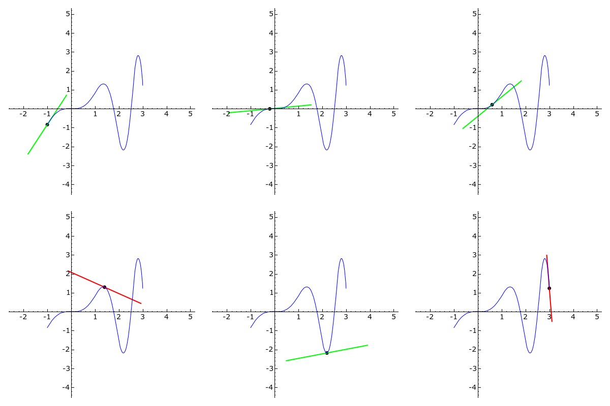
The derivative f′ of a univariate function f tells us the instantaneous rate of change at a given point x; it provides a measurement of how much f increases or decreases.

A gradient is the generalization of the derivative to multi-variate functions; it is a vector of the function’s partial derivatives. A partial derivative of a function is the derivative (instantaneous rate of change) with respect to only one of its variables, and considering the others as constants. The gradient of a function is the vector of all of the functions partial derivatives. The gradient of a scalar function denotes the direction of greatest change.

Gradient Descent is a powerful and generic optimization algorithm. It works by iteratively tweaking a model’s parameters in the cost function’s direction of greatest change (the gradient). Because we are interested in minimizing the cost function, we apply the update in the opposite direction of the gradient (in other words, the negative gradient).

NOTE: Because it works using only gradient (first derivative) information, Gradient Descend is called a first-order optimization method. Other methods use Hessian (second derivative) information and may converge much faster (for example, Newton’s method). Computing the Hessian is extremely costly, however. This prevents their use with large models such as Deep Neural Networks.

Learning Rate Effects

Gradient Descent applies the learning rate as a scaling term to the negative gradient. It controls the magnitude of the weight updates. The figure below visualizes the training loss of models trained on the CIFAR10 dataset using different learning rates.

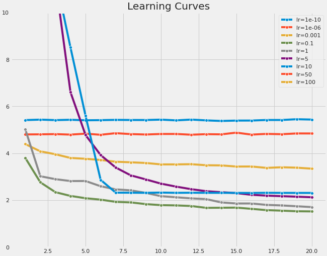
Using a very large learning rate can result in large loss values. Although the loss will decrease, it will remain significantly higher than the loss obtained using a smaller, more adequate learning rate. For more extreme cases, large learning rates can lead to divergence, wildly shooting around and never settling to a stable configuration. Conversely, if the learning rate is too small, training can be extremely slow.

The learning rate is commonly denoted with the Greek letter η (eta) in the Deep Learning literature.

Learning Rate Initialization and Scheduling

As we saw in the previous section, the choice of learning rate can drastically impact the quality of the solution reached. In the sections below, I will present a simple and effective learning rate initialization technique. I will then present a learning rate schedule, used to dynamically modify the learning rate during training and achieve even faster convergence.

NOTE: The code used was adapted from Chapter 11 of “Hands-On Machine Learning with Scikit-Learn, Keras, and TensorFlow”. You can find the original notebook here.

Exponential Increments

The first technique is to train your model for a few hundred iterations, beginning with a very small learning rate (for example, 1e-6), and gradually incrementing it exponentially, up to a large value (for example, 10). The optimal learning rate would be approximately 10 times less than the point before the loss starts to shoot up. A Keras implementation of the exponential increase technique can be found below.

The learning rate found using the approach described above will be used as a threshold for a more effective technique used to dynamically modify the learning rate during training.

1cycle Scheduling

Instead of using a constant learning rate, we can dynamically modify the learning rate during training. When used appropriately, this technique leads to good solutions and faster convergence. A schedule is a strategy used to modify the learning rate. In 2018, Leslie Smith proposed the 1cycle schedule, a simple and effective schedule where the learning rate is increased during the first half of training, then decreased in the second half. The 1cycle schedule works as follows:

1. Initialize η to some initial value η0
2. Linearly increase η, reaching the maximum η1 halfway through training
3. Linearly decrease η, going down to η0. The last iterations should drop η by several orders of magnitude

The maximum η1 can be selected via the Exponential Increase method presented above. The initial learning rate η0 can be set to be roughly 10 times lower than η1.

Below is a Keras implementation of 1cycle scheduling:

Experimental Results

The following section presents my experimental results. For image classification tasks on CIFAR10 and Fashion MNIST, I trained a Convolutional Neural Network with the following architecture:

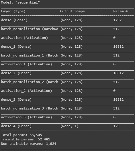
For the Boston Housing dataset, I trained a model with the following architecture:

All tasks use a batch size of 32.

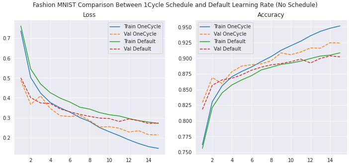
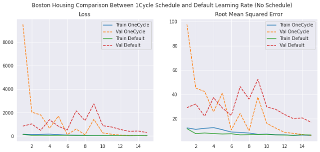
Conclusion

In this article I presented the 1cycle learning rate schedule. When tuned appropriately, this technique yielded significantly improved task performance while converging faster. There is, however, some tuning required. In particular, I found the batch size, initial, and maximum learning rate to require careful selection. Once sensible values are found, however, the benefit of using 1cycle scheduling is clear.

Important: Batch size played a crucial role in these experiments. A batch size of 32 yielded quite favorable results, at the expense of slightly lower training times. However, using large batch sizes such as 2048 resulted in exploding weight updates and Nan values.

Finally, do not forget to scale your data. One common and effective scaling method is to standardize the data to zero mean and unit variance. For a more in-depth explanation on the importance of preserving variance across the Neural Network, check out this article.

Sources

• https://www.jmlr.org/papers/volume13/bergstra12a/bergstra12a.pdf
• https://en.wikipedia.org/wiki/Bayesian_optimization
• https://ai.googleblog.com/2019/05/efficientnet-improving-accuracy-and.html
• Hands-on Machine Learning with Scikit-Learn, Keras and TensorFlow Ch11
• A disciplined approach to neural network hyper-parameters: Part 1 — learning rate, batch size, momentum, and weight decay
• https://en.wikipedia.org/wiki/Standard_score
• https://pub.towardsai.net/solving-the-vanishing-gradient-problem-with-self-normalizing-neural-networks-using-keras-59a1398b779f

Join thousands of data leaders on the AI newsletter. Join over 80,000 subscribers and keep up to date with the latest developments in AI. From research to projects and ideas. If you are building an AI startup, an AI-related product, or a service, we invite you to consider becoming a sponsor.

Published via Towards AI