Deep Learning from Scratch in Modern C++: Cost Functions

Author(s): Luiz doleron

Originally published on Towards AI.

Let’s have fun by implementing Cost Functions in pure C++ and Eigen.

In machine learning, we usually model problems as functions. Therefore, most of our work consists of finding ways to approximate functions using well-known models. In this context, Cost Functions play a central role.

This story is a sequel to our previous talk about convolutions. Today, we will introduce the concept of cost functions, show common examples and learn how to code and plot them. As always, from scratch in pure C++ and Eigen.

About this series

In this series, we will learn how to code the must-to-know deep learning algorithms such as convolutions, backpropagation, activation functions, optimizers, deep neural networks, and so on using only plain and modern C++.

This story is: Cost functions in C++

Check other stories:

0 — Fundamentals of deep learning programming in Modern C++

1 — Coding 2D convolutions in C++

3 — Implementing Gradient Descent

4 — Activation Functions

… more to come.

Modeling in machine learning

As artificial intelligence engineers, we usually define every task or problem as a function.

For example, if we are working on a face recognition system, our first step is to define the problem as a function to map an input image to an identifier:

For a medical diagnosis system, we can define a function to map symptoms to diagnostics:

We can write a model to provide an image given a sequence of words:

This is an endless list. Using functions to represent tasks or problems is the streamlined way to implement machine learning systems.

The problem often is: how to know the F() formula?

Approximating Functions

Indeed, defining F(X) using a formula or a sequence of rules is not feasible (one day I shall explain why).

In general, instead of finding or defining the proper function F(X), we try to find an approximation of F(X). Let’s call this approximation by hypothesis function, or simply, H(X).

At first glance, it does not make sense: if we need to find the approximation function H(X), why do we not try to find F(X) directly?

The answer is: we know H(X). Whereas we do not know much about F(X), we know almost everything about H(X): its formula, parameters, etc. The only thing we don’t know about H(X) are its parameter values.

Indeed, the main concern in machine learning is finding ways to determine suitable parameter values for a given problem and data. Let’s see how we can carry it out.

In machine learning terminology, H(X) is said “an approximation of F(X)”. The existence of H(X) is covered by the Universal Approximation Theorem.

Cost Function and The Universal Approximation Theorem

Consider the case where we know the value of the input Xand the respective output Y = F(X) but we do not know the formula of F(X). For example, we know that if the input isX = 1.0 then F(1.0)results inY = 2.0.

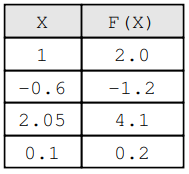
Now, consider that we have a known function H(X) and we are wondering whetherH(X) is a good approximation for F(X). Thus, we calculate T = H(1.0) and find T = 1.9 .

How bad is this value T = 1.9 since we know that the true value is Y = 2.0 when X = 1.0?

The metric to quantify the cost of the difference between Y and T is called by Cost Function.

Note that Y is the expected value and T is the actual value obtained by our guess H(X)

The concept of cost functions is core in machine learning. Let’s introduce the most common cost function as an example.

Mean Squared Error

The most known cost function is the Mean Squared Error:

where Tᵢ is given by the convolution of Xᵢ by kernel k:

We discussed Convolution in the previous story

Note that we have n pairs (Yₙ, Tₙ) each one a combination of the expected value Yᵢ and the actual value Tₙ. For example:

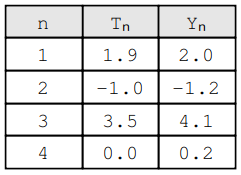
Hence, MSE is evaluated as follows:

We can write our first version of MSE as follows:

auto MSE = [](const std::vector<double> &Y_true, const std::vector<double> &Y_pred) {

 if (Y_true.empty()) throw std::invalid_argument("Y_true cannot be empty.");

 if (Y_true.size() != Y_pred.size()) throw std::invalid_argument("Y_true and Y_pred sizes do not match.");

 auto quadratic = [](const double a, const double b) {
 double result = a - b;
 return result * result;
 };
 const int N = Y_true.size();
 double acc = std::inner_product(Y_true.begin(), Y_true.end(), Y_pred.begin(), 0.0, std::plus<>(), quadratic);

 double result = acc / N;

 return result;
};

Now we know how to calculate MSE, let’s see how to use it to approximate functions.

The intuition of using MSE to find the best parameters

Let’s assume that we have a mapping F(X) synthetically generated by:

F(X) = 2*X + N(0, 0.1)

where N(0, 0.1) represents a random value drawn from the normal distribution with mean = 0 and standard deviation = 0.1. We can generate sample data by:

#include <random>

std::default_random_engine dre(time(0));

std::normal_distribution<double> gaussian_dist(0., 0.1);
std::uniform_real_distribution<double> uniform_dist(0., 1.);

std::vector<std::pair<double, double>> sample(90);

std::generate(sample.begin(), sample.end(), [&gaussian_dist, &uniform_dist]() {
 double x = uniform_dist(dre);
 double noise = gaussian_dist(dre);
 double y = 2. * x + noise;
 return std::make_pair(x, y);
});

If we plot this sample using any spreadsheet software, we get something like this:

Note that we know the formula of G(X) and F(X). In real life, however, these generator functions are undisclosed secrets of the underlying phenomena. Here, in our example, we only know them because we are generating synthetic data to help us to get a better understanding.

In real life, everything we know is an assumption that the hypothesis function H(X) defined by H(X) = kX might be a good approximation of F(X). Of course, we don’t know what is the value of k yet.

Let’s see how to use MSE to find out a suitable value of k. Indeed, it is as simple as plotting MSE for a range of different k’s:

std::vector<std::pair<double, double>> measures;

double smallest_mse = 1'000'000'000.;
double best_k = -1;
double step = 0.1;

for (double k = 0.; k < 4.1; k += step) {
 std::vector<double> ts(sample.size());
 std::transform(sample.begin(), sample.end(), ts.begin(), [k](const auto &pair) {
 return pair.first * k;
 });

 double mse = MSE(ys, ts);
 if (mse < smallest_mse) {
 smallest_mse = mse;
 best_k = k;
 }

 measures.push_back(std::make_pair(k, mse));
}

std::cout << "best k was " << best_k << " for a MSE of " << smallest_mse << "\n";

Very often, this program outputs something like this:

best k was 2.1 for a MSE of 0.00828671

If we plot MSE(k) by k, we can see a very interesting fact:

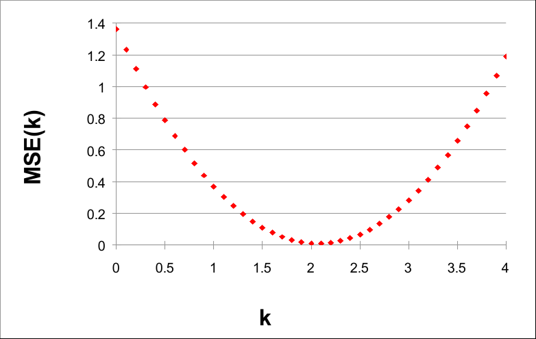
Note that the value of MSE(k) is minimum in the neighborhood of k = 2. Indeed, 2 is the parameter of the generatrix function G(X) = 2X.

Given the data and using steps of 0.1, the smaller value of MSE(k) is found when k = 2.1. This suggests that H(X) = 2.1X is a good approximation of F(X). In fact, if we plot, F(X), G(X), and H(X), we have:

By the chart above, we can realize that H(X) actually approximates F(X). We can try using smaller steps like 0.01 or 0.001 to find a better approximation, though.

The code can be found on this repository

The Cost Surface

The curve of MSE(k) by k is a one-dimensional example of the Cost Surface.

What the previous example shows is that we can use the minimum value of the cost surface to find the best fit for the parameter k.

The example describes the most important paradigm in machine learning: functions approximations by cost function minimization.

The previous chart shows a 1-dimensional cost surface, i.e., a cost curve given a single-dimensional k. In 2-D spaces, i.e., when we have two k’s namely k0 and k1, the cost surface looks more like an actual surface:

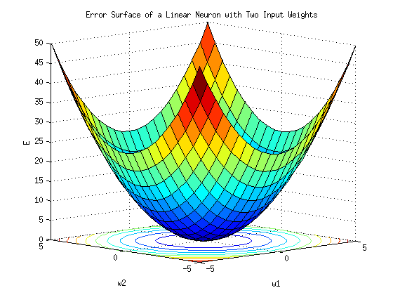
Regardless of whether k is 1D, 2D, or even higher-dimensional, the process of finding the best k-th values is the same: finding the smallest value of the cost curve.

The smallest cost value is also known as Global Minima.

In 1D spaces, the process of finding the global minima is relatively easy. However, on high dimensions, scanning all space to find the minima can be computationally costly. In the next story, we will introduce algorithms to perform this search at scale.

Not only k can be high-dimensional. In real problems, very often the outputs are high-dimensional too. Let’s learn how to calculate MSE in cases like this.

MSE on High-Dimensional Outputs

In real-world problems, Y and T are vectors or matrices. Let’s see how to deal with data like this.

If the output is single-dimensional, the previous formula of MSE will work out. But if the output is multi-dimensional, we need to change the formula a little bit. For example:

In this case, instead of scalar values, Yₙ and Tₙ are matrices of size (2,3). Before applying MSE to this data, we need to change the formula as follows:

In this formula, N is the number of pairs, R is the number of rows, and C is the number of columns in each pair. As usual, we can implement this version of MSE using lambdas:

#include <numeric>
#include <iostream>

#include <Eigen/Core>

using Eigen::MatrixXd;

int main() 
{

 auto MSE = [](const std::vector<MatrixXd> &Y_true, const std::vector<MatrixXd> &Y_pred) 
 {

 if (Y_true.empty()) throw std::invalid_argument("Y_true cannot be empty.");

 if (Y_true.size() != Y_pred.size()) throw std::invalid_argument("Y_true and Y_pred sizes do not match.");

 const int N = Y_true.size();
 const int R = Y_true[0].rows();
 const int C = Y_true[0].cols();

 auto quadratic = [](const MatrixXd a, const MatrixXd b) 
 {
 MatrixXd result = a - b;
 return result.cwiseProduct(result).sum();
 };

 double acc = std::inner_product(Y_true.begin(), Y_true.end(), Y_pred.begin(), 0.0, std::plus<>(), quadratic);

 double result = acc / (N * R * C);

 return result;
 };

 std::vector<MatrixXd> A(4, MatrixXd::Zero(2, 3)); 
 A[0] << 1., 2., 1., -3., 0, 2.;
 A[1] << 5., -1., 3., 1., 0.5, -1.5; 
 A[2] << -2., -2., 1., 1., -1., 1.; 
 A[3] << -2., 0., 1., -1., -1., 3.;

 std::vector<MatrixXd> B(4, MatrixXd::Zero(2, 3)); 
 B[0] << 0.5, 2., 1., 1., 1., 2.; 
 B[1] << 4., -2., 2.5, 0.5, 1.5, -2.; 
 B[2] << -2.5, -2.8, 0., 1.5, -1.2, 1.8; 
 B[3] << -3., 1., -1., -1., -1., 3.5;

 std::cout << "MSE: " << MSE(A, B) << "\n";

 return 0;
}

It is noteworthy that, regardless k or Y are or are not multi-dimensional, MSE is always a scalar value.

Other Cost Functions

In addition to MSE, other cost functions are also regularly found in deep learning models. The most commons are categorial cross-entropy, log cosh, and cosine similarity.

We will cover these functions in forthcoming stories, in particular when we cover classification and non-linear inference.

Conclusion and Next Steps

Cost Functions are one of the most important topics in machine learning. In this story, we learned how to code MSE, the most used cost function, and how to use it to fit single-dimensional problems. We also learned why cost functions are so important to find function approximations.

In the next story, we will learn how to use cost functions to train convolution kernels from data. We will introduce the base algorithm to fit kernels and discuss the implementation of training mechanics such as epochs, stop conditions, and hyperparameters.

Join thousands of data leaders on the AI newsletter. Join over 80,000 subscribers and keep up to date with the latest developments in AI. From research to projects and ideas. If you are building an AI startup, an AI-related product, or a service, we invite you to consider becoming a sponsor.

Published via Towards AI