The Intuition Behind GANs for Beginners

Author(s): Sushant Gautam

Originally published on Towards AI the World’s Leading AI and Technology News and Media Company. If you are building an AI-related product or service, we invite you to consider becoming an AI sponsor. At Towards AI, we help scale AI and technology startups. Let us help you unleash your technology to the masses.

Deep Learning

You have probably heard about deep fake videos or visit thispersondoesnotexit, where GAN is used to create those. Isn’t that Interesting. In this post, we will discuss the basic intuition behind GAN in-depth, its implementation in Tensorflow. Let’s get started.

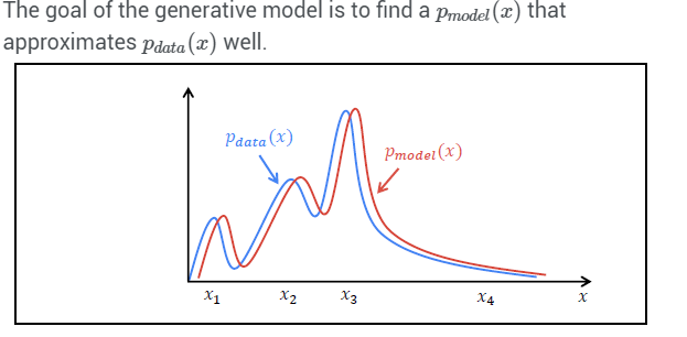
Generative Adversarial Networks, in short, GAN are an approach to generative modeling using deep learning methods, such as Convolutional Neural Networks. Generative modeling is an unsupervised learning task in machine learning where the goal is to find the hidden patterns in the input data and produce plausible images having similar characteristics to input data.

GAN is able to learn how to model the input distribution by training two competing (and cooperating) networks referred to as generator and discriminator(also known as a critic). The task of the generator is to keep figuring out how to generate fake data or signals that can fool the discriminator. Initially, some noise input is given to the generator to work on it. On the other hand, a discriminator is trained to distinguish between fake and real signals.

The main concept of GAN is straightforward. The GAN model architecture involves two sub-models: a generator model for generating new examples and a discriminator model for classifying whether generated examples are real (from the domain) or fake (generated by the generator model). Let’s take a look at it as:

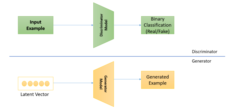
• Discriminator: Model that learns how to classify input as real(from the domain) or fake(generated).
• Generator: Model that generates new similar images from the problem domain.

How does GAN work?

The two neural networks that make up the GAN are called the generator and the discriminator. The GAN generator generates new data instances and the discriminator validates, or whether they belong in the dataset (real) or generated(fake). The discriminator is a fully connected neural network that classifies the input example as real(1.0) or fake(0.0). At regular intervals, the generator will pretend that its output is genuine data and will ask the discriminator to label it as 1.0. When the fake data is then presented to the
discriminator, naturally it will be classified as fake with a label close to 0.0.

Overall, the whole process is that two networks compete with one another while still cooperating with each other. In the end, when the GAN training converges, the end result is a generator that can generate plausible data that appears to be real. The discriminator thinks this synthesized data is real and labels it as 1.0.

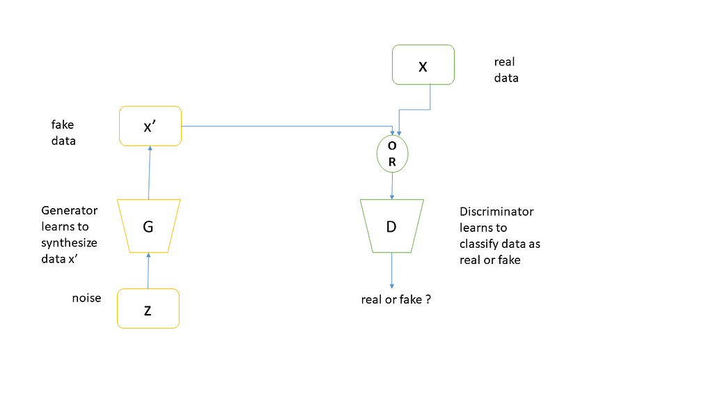
The input to the generator is noise, and the output is synthesized data. Meanwhile, the discriminator’s input will either be real or synthesized data. Real data comes from the true sampled data, while the fake data comes from the generator. All the real data is labeled 1.0 (i.e 100% probability of being real), while all the synthesized data (fake data) is labeled 0.0 (i.e 0% probability of being real). Here is an algorithm from the authors of GAN:

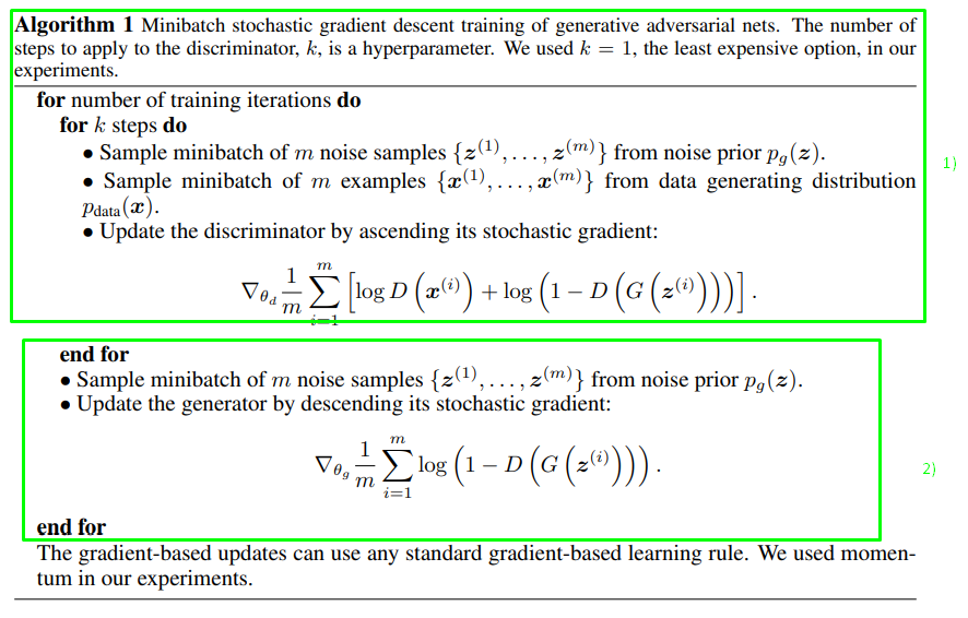
As you can see, the Discriminator is updated for k steps and only then the Generator is updated. This process is repeated continuously. k can be set to 1, but usually larger values are better (Goodfellow et al., 2014). Any gradient-based learning rule can be used for optimization.

The Loss function shown in the above algorithm is called Minmax Loss. Since the generator tries to minimize the function while the discriminator tries to maximize it. It can be written as:

Some notation is:

D(x) →Probability that the given real data instance x is real by the discriminator.

Eₓ → Expected value overall instances.

G(z) → Generator output gave the noise vector z.

D(G(z)) → Probability that the given fake data instance z is real by the discriminator.

E𝓏 → Expected value overall generated fake instances.

The generator can’t directly affect the log(D(x)) term in the function, so, for the generator, minimizing the loss is equivalent to minimizing log(1 – D(G(z))) .

In summary the difference between generative and discriminative models:

• A discriminative model learns a function that maps the input data (x) to some desired output class label (y). In probabilistic terms, they directly learn the conditional distribution P(y|x).
• A generative model tries to learn the joint probability of the input data and labels simultaneously, i.e. P(x,y). This can be converted to P(y|x) for classification via the Bayes rule, but the generative ability could be used for something else as well, such as creating likely new (x, y) samples.

Training Discriminator

The discriminator connects to two loss functions. During discriminator training, the discriminator ignores the generator loss and just uses the discriminator loss. We use the generator loss during generator training.

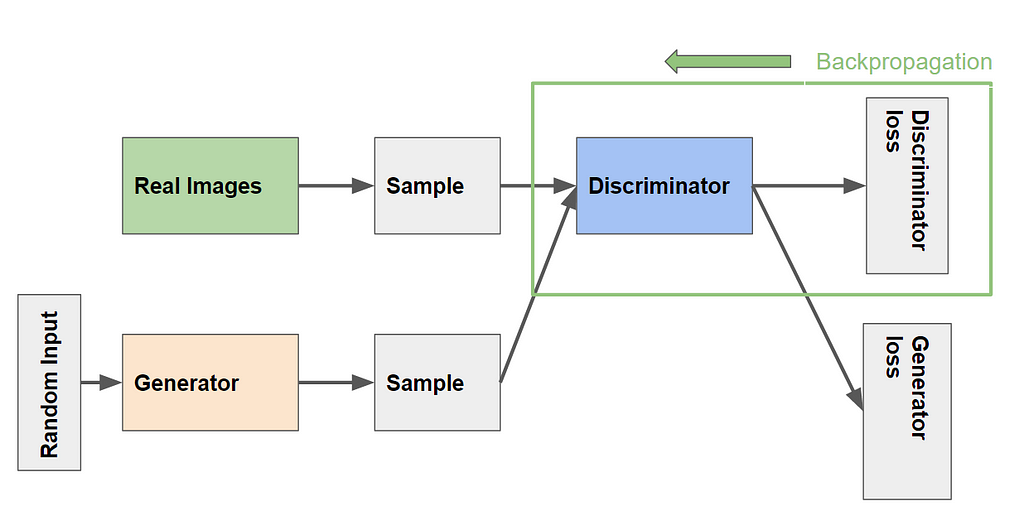
The discriminator’s training data comes from two sources:

• Real data instances, such as real pictures of people. The discriminator uses these instances as positive examples during training.
• Fake data instances created by the generator. The discriminator uses these instances as negative examples during training.

In the given figure above, the two “Sample” boxes represent these two data sources feeding into the discriminator. During discriminator training, the generator does not train. Its weights remain fixed while it produces examples for the discriminator to train on.

During discriminator training:

1. The discriminator classifies both real data and fake data from the generator.
2. The discriminator loss penalizes the discriminator for misclassifying a real instance as fake or a fake instance as real.
3. The discriminator updates its weights through backpropagation from the discriminator loss through the discriminator network.

Training Generator

The generator part of a GAN learns to create fake data by taking feedback from the discriminator. Feedback from the discriminator helps the generator to improve its output over time. It learns to make the discriminator classify its output as real.

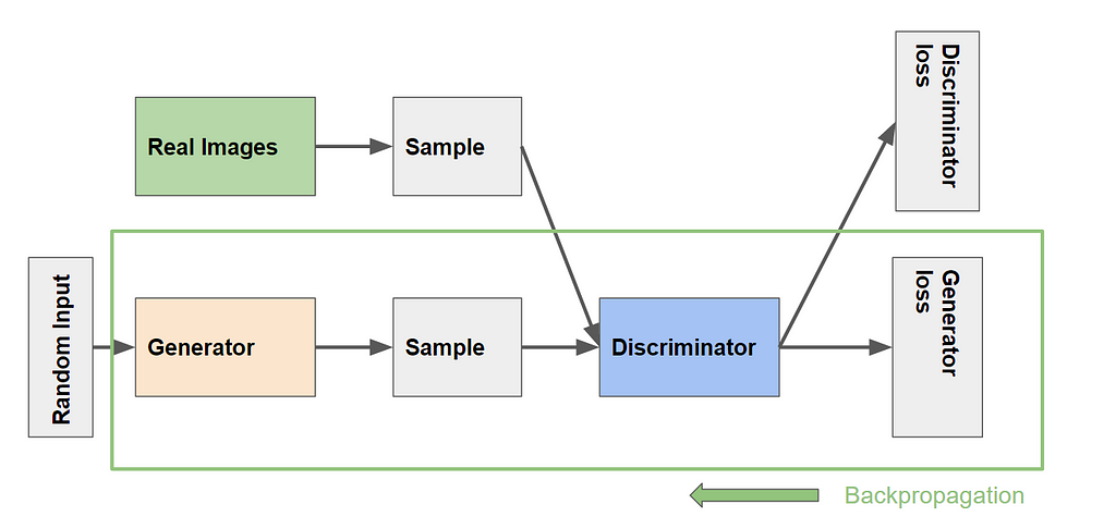
The above figure depicts the training of the generator. It involves a combination of discriminator and generator. The output of the generator is passed to the discriminator net, and the discriminator compares to real output and output loss. The generator loss penalizes the generator for producing a sample that the discriminator network classifies as fake.

Backpropagation adjusts each weight in the right direction by calculating the weight’s impact on the output. Discriminator parameters are frozen but gradients are passed down to the Generator. So backpropagation starts at the output and flows back through the discriminator into the generator.

Generator training requires tighter integration between the generator and the discriminator than discriminator training requires. One iteration of training the generator involves the following procedure:

1. Sample random noise.
2. Produce generator output from sampled random noise.
3. Get discriminator “Real” or “Fake” classification for generator output.
4. Calculate loss from discriminator classification.
5. Backpropagate through both the discriminator and generator to obtain gradients.
6. Use gradients to change only the generator weights. (Discriminator weights are frozen)

Pseudocode of Training GAN:

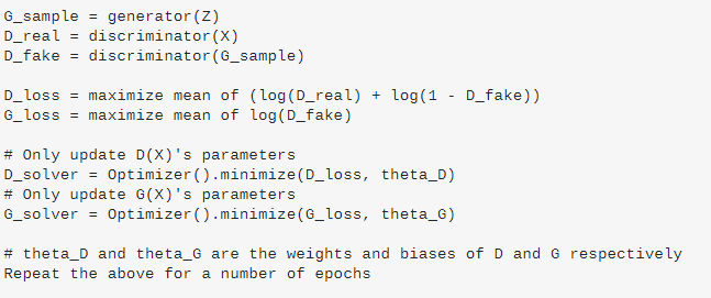
Now you understand the basic intuition of GAN. Let's try to implement a DCGAN in Tensorflow 2.

Simple DC GAN in Tensorflow 2

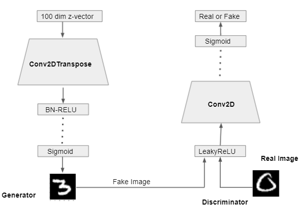
The generator accepts 100 dim z-vector noise sampled from a uniform distribution. Then many layers of Conv2DTranspose with Batch Normalization and RELU activation function is used. Basically, Conv2DTranspose up sample image from 100 dim vectors to the given shape. Batch Normalization is used for convergence and fast training. The final layer has sigmoid activation, which generates the 28 x 28 x 1 fake MNIST images.

CODE:

Complete code is found in this Collab notebook link.

The discriminator is similar to the CNN image classifiers. It takes a 28x28x1 image. It takes both real and fake images and concatenates them. It consists of layers of CONV2D with a leakyRELU activation function. The final layer is the sigmoid which outputs 1(REAL) of 0(FAKE) output.

Firstly, the discriminator model is built, and, following that, the generator model is instantiated. Finally, we combine both discriminator and generator as adversarial models and train them.

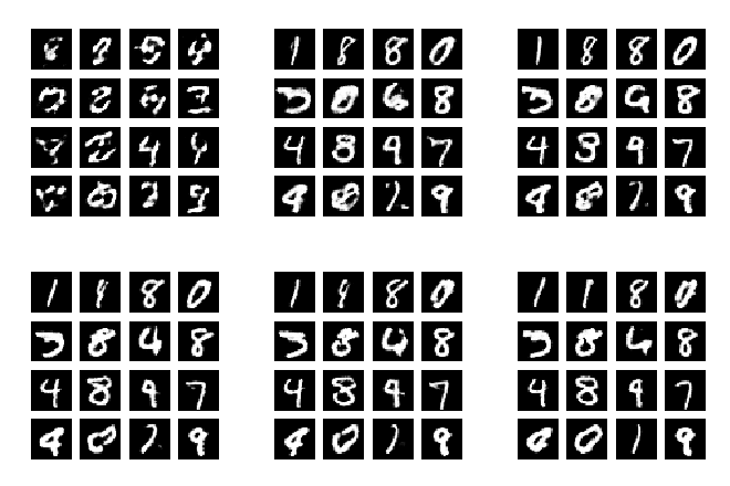
Output:

References

[1] Goodfellow, Ian, et al. “Generative adversarial nets.” Advances in neural information processing systems. 2014.

[2] Atienza, Rowel. Advanced Deep Learning with Tensorflow 2 and Keras: Apply DL, Gans, Vaes, Deep RL, Unsupervised Learning, Object Detection and Segmentation, and More. Packt Publishing Ltd., 2020.

If you like it, please share and click the green icon which I appreciate a lot.

---

The Intuition Behind GANs for Beginners was originally published in Towards AI on Medium, where people are continuing the conversation by highlighting and responding to this story.

Join thousands of data leaders on the AI newsletter. It’s free, we don’t spam, and we never share your email address. Keep up to date with the latest work in AI. From research to projects and ideas. If you are building an AI startup, an AI-related product, or a service, we invite you to consider becoming a sponsor.

Published via Towards AI