Regression Line with Mathematics for the Linear Regression

Last Updated on July 9, 2020 by Editorial Team

Author(s): Gul Ershad

Statistics

Introduction

Regression is a prediction where the target is continuous and its applications are several. It is the simplest parametric model. Every data-set is given in a pair consisting of an input feature vector and label value. The main goal is to hypothesize the parameters to predict the target values of the test data after training from the training data-set.

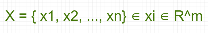
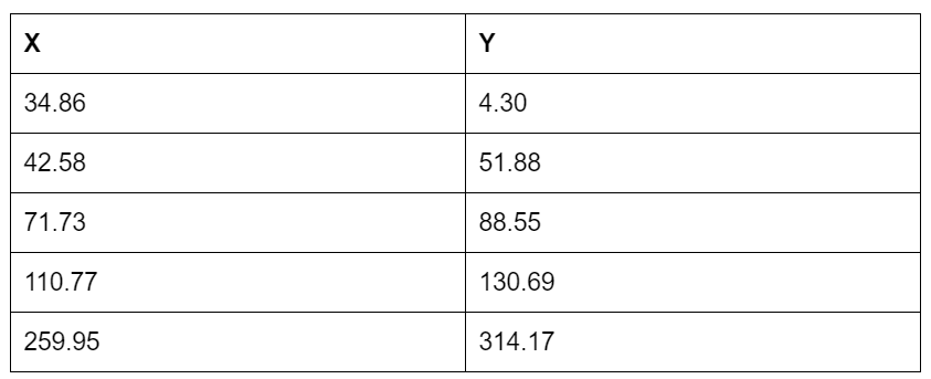
The below table has two variables X and Y. Here, Y is known as the target variable or independent variable, and X is known as the explanatory variable.

The prediction of the height of a child based on his age and weight can be an example of a regression problem.

Lets X is a real-values:

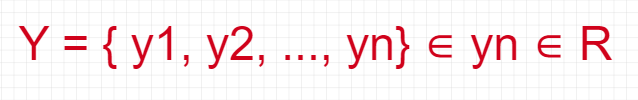
And, the real value of Y:

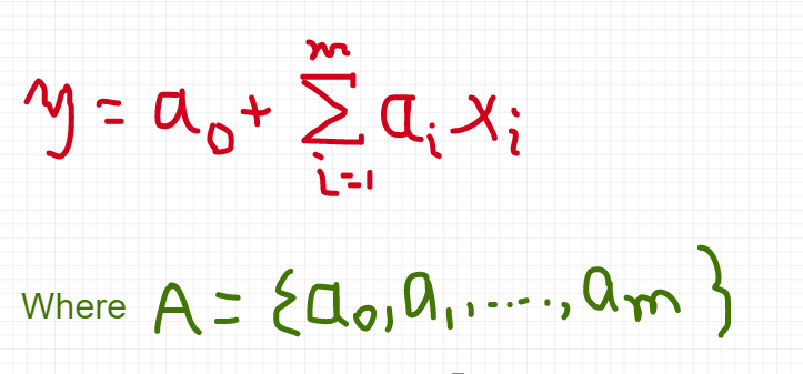
So, the regression process based on the given rule:

Approach to Regression

Following are the general approach to Regression:

1. Collect data
2. Prepare data: Numeric values should be there for the regression. If there are nominal values, it should be mapped to binary values.
3. Analysis: Good for the visualization into 2D plots.
4. Train: Find the regression weights.
5. Test: Measure the R2, or correlation of the predicted values and data. It measures the accuracy of the model.

Regression Line

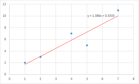
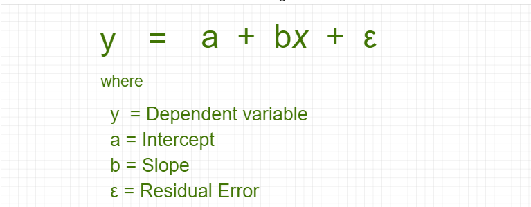
Linear regression consists of finding the best-fitting straight line through the points. The best-fitting line is called a regression line.

The equation of Regression Line:

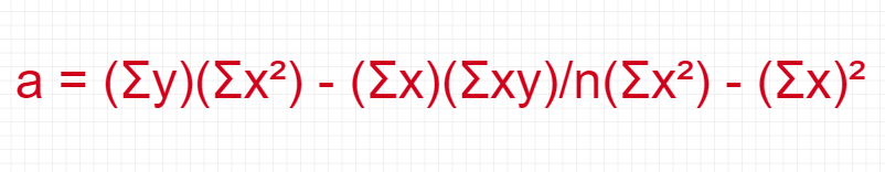
The equation of Intercept a:

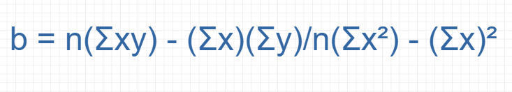
The equation of Slope b:

Properties of Regression Line

The regression line has the following properties:

1. The regression always runs and rise through points x and y mean.
2. This line minimizes the sum of square differences between observed values and predicted values.
3. In the regression line, x is the input value and y is the output value.

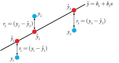
Residual Error in Regression Line

Residual Error is the difference between the observed value of the dependent value and predicted value.

Residual Error = Observed value – Predicated value

Derivative to find the equation of Regression Line

Let’s consider the following variables x and y with their values:

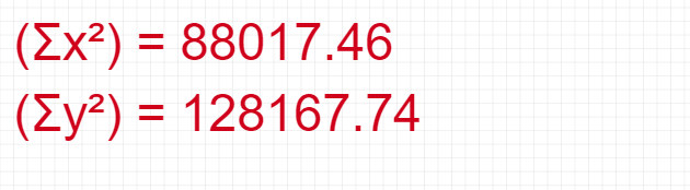
So, to calculate the values of a and b lets find the values of XY, X², and Y².

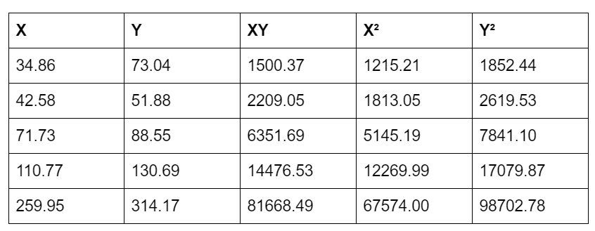
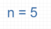
Here,

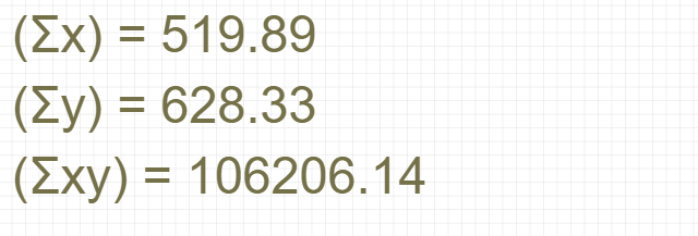
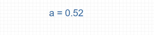
Now, find the value of Intercept a :

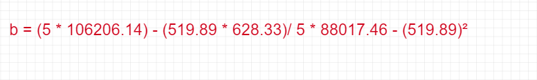
Find the value of Slope b:

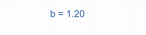
Hence, the Regression Line equation:

Linear Regression

Let's take an example, try to forecast the horsepower of a friend’s automobile so its equation will be:

Horsepower = 0.0018 * annual_salary — 0.99*hourslistening_radio

This equation is known as a regression equation. The values of 0.0018 and 0.99 are known as regression weights. And, the process of finding these regression weights is called regression.

Forecasting new values given set of input is easy once the regression weights are found.

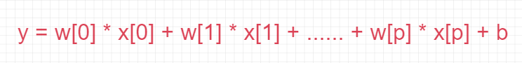
For regression, the prediction formula for the linear regression is like below:

import mglearn

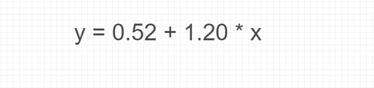
mglearn.plots.plot_linear_regression_wave()

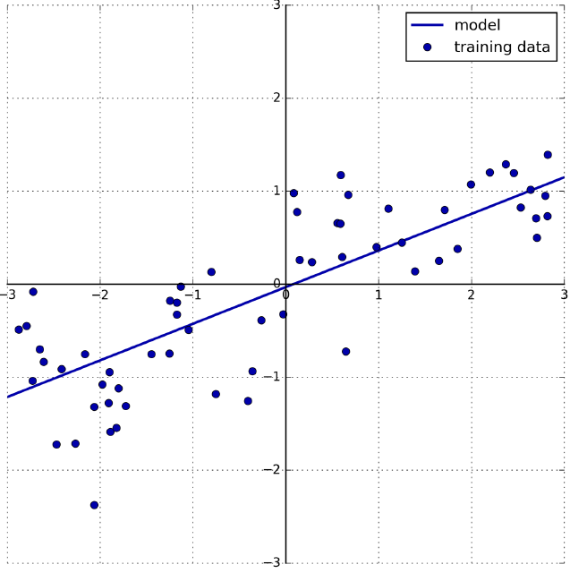
There are many different linear models for regression. The difference between these models lies in how the model parameters w and b are learned from the training data, and how model complexity can be controlled.

Pros of Linear Regression:

1. It easy to interpret and computationally inexpensive

Cons of Linear Regression:

1. It poorly models on non-linear data

Conclusion

To find the best-fitting straight line through the points is an important part of Linear regression and this line is called a regression line. Linear regression consists of finding the best-fitting straight line through the points. The least-squares method is used to find the best-fitting straight line in regression.

References

Introduction to Linear Regression: http://onlinestatbook.com/2/regression/introC.html

---

Regression Line with Mathematics for the Linear Regression was originally published in Towards AI — Multidisciplinary Science Journal on Medium, where people are continuing the conversation by highlighting and responding to this story.

Published via Towards AI