


Decision Trees Explained With a Practical Example
Last Updated on January 6, 2023 by Editorial Team
Author(s): Davuluri Hemanth Chowdary
A decision tree is one of the supervised machine learning algorithms. This algorithm can be used for regression and classification problems — yet, is mostly used for classification problems. A decision tree follows a set of if-else conditions to visualize the data and classify it according to the conditions.
For example,
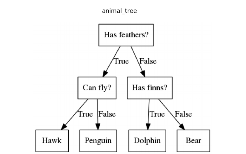
Before we dive deep into the decision tree’s algorithm’s working principle, you need to know a few keywords related to it.
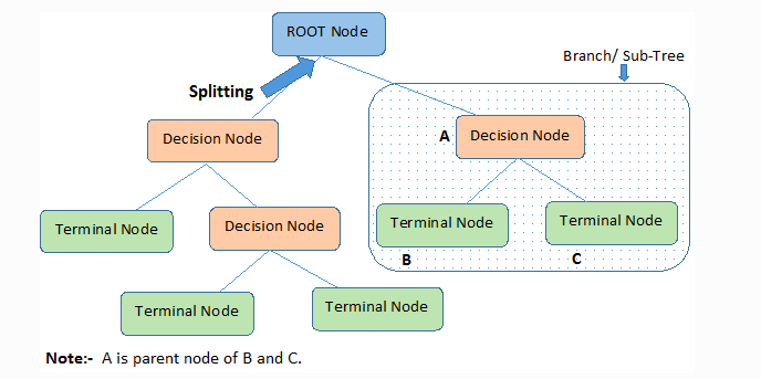
Important terminology
- Root Node: This attribute is used for dividing the data into two or more sets. The feature attribute in this node is selected based on Attribute Selection Techniques.
- Branch or Sub-Tree: A part of the entire decision tree is called a branch or sub-tree.
- Splitting: Dividing a node into two or more sub-nodes based on if-else conditions.
- Decision Node: After splitting the sub-nodes into further sub-nodes, then it is called the decision node.
- Leaf or Terminal Node: This is the end of the decision tree where it cannot be split into further sub-nodes.
- Pruning: Removing a sub-node from the tree is called pruning.
Working of Decision Tree
- The root node feature is selected based on the results from the Attribute Selection Measure(ASM).
- The ASM is repeated until a leaf node, or a terminal node cannot be split into sub-nodes.
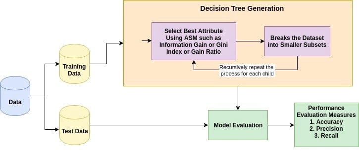
What is Attribute Selective Measure(ASM)?
Attribute Subset Selection Measure is a technique used in the data mining process for data reduction. The data reduction is necessary to make better analysis and prediction of the target variable.
The two main ASM techniques are
- Gini index
- Information Gain(ID3)
Gini index
The measure of the degree of probability of a particular variable being wrongly classified when it is randomly chosen is called the Gini index or Gini impurity. The data is equally distributed based on the Gini index.
Mathematical Formula :
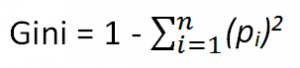
Pi= probability of an object being classified into a particular class.
When you use the Gini index as the criterion for the algorithm to select the feature for the root node.,The feature with the least Gini index is selected.
Information Gain(ID3)
Entropy is the main concept of this algorithm, which helps determine a feature or attribute that gives maximum information about a class is called Information gain or ID3 algorithm. By using this method, we can reduce the level of entropy from the root node to the leaf node.
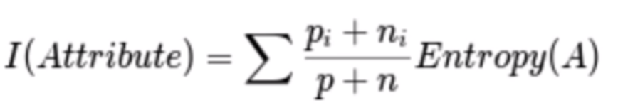
Mathematical Formula :
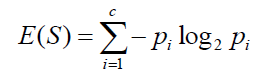
‘p’, denotes the probability of E(S), which denotes the entropy. The feature or attribute with the highest ID3 gain is used as the root for the splitting.
Well, I know the ASM techniques are not clearly explained in the above context.
Let me explain the whole process with an example.
IT’S TIME FOR PRACTICAL EXAMPLE
Problem Statement:
Predict the loan eligibility process from given data.
The above problem statement is taken from Analytics Vidhya Hackathon.
You can find the dataset and more information about the variables in the dataset on Analytics Vidhya.
I took a classification problem because we can visualize the decision tree after training, which is not possible with regression models.
Step1: Load the data and finish the cleaning process
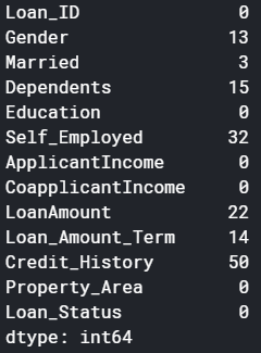
There are two possible ways to either fill the null values with some value or drop all the missing values(I dropped all the missing values).
If you look at the original dataset’s shape, it is (614,13), and the new data-set after dropping the null values is (480,13).
Step 2: Take a Look at the data-set
We found there are many categorical values in the dataset.
NOTE: The decision tree does not support categorical data as features.
So the optimal step to take at this point is you can use feature engineering techniques like label encoding and one hot label encoding.
Step 3: Split the data-set into train and test sets
Why should we split the data before training a machine learning algorithm?
Please visit Sanjeev’s article regarding training, development, test, and splitting of the data for detailed reasoning.
Step 4: Build the model and fit the train set.
Before we visualize the tree, let us do some calculations and find out the root node by using Entropy.
Calculation 1: Find the Entropy of the total dataset
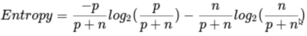
p = no of positive cases(Loan_Status accepted)
n = number of negative cases(Loan_Status not accepted)
In the data set, we have
p = 332 , n=148, p+n=480
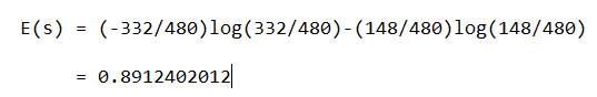
here log is with base 2
Entropy = E(s) = 0.89
Calculation 2: Now find the Entropy and gain for every column
1) Gender Column

There are two types in this male(1) and female(0)
Condition 1: Male
data-set with all male’s in it and then,
p = 278, n=116 , p+n=489
Entropy(G=Male) = 0.87
Condition 2: Female
data-set with all female’s in it and then,
p = 54 , n = 32 , p+n = 86
Entropy(G=Female) = 0.95
Average Information in Gender column is

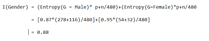
Gain

Gain(Gender) = E(s) — I(Gender)
Gain = 0.89–0.88
Gain = 0.001
2) Married Column

In this column we have yes and no values
Condition 1: Married = Yes(1)
In this split the whole data-set with Married status yes
p = 227 , n = 84 , p+n = 311
E(Married = Yes) = 0.84
Condition 2: Married = No(0)
In this split the whole data-set with Married status no
p = 105 , n = 64 , p+n = 169
E(Married = No) = 0.957
Average Information in Married column is
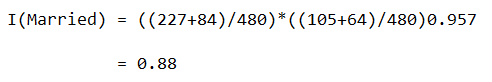
Gain = 0.89–0.88 = 0.001
3) Education Column

In this column, we have graduate and not graduate values.
Condition 1: Education = Graduate(1)
p = 271 , n = 112 , p+n = 383
E(Education = Graduate) = 0.87
Condition 2: Education = Not Graduate(0)
p = 61 , n = 36 , p+n = 97
E(Education = Not Graduate) = 0.95
Average Information of Education column= 0.886
Gain = 0.01
4) Self-Employed Column

In this column we have Yes or No values
Condition 1: Self-Employed = Yes(1)
p = 43 , n = 23 , p+n = 66
E(Self-Employed=Yes) = 0.93
Condition 2: Self-Employed = No(0)
p = 289 , n = 125 , p+n = 414
E(Self-Employed=No) = 0.88
Average Information in Self-Employed in Education Column = 0.886
Gain = 0.01
5) Credit Score Column

In this column we have 1 and 0 values
Condition 1: Credit Score = 1
p = 325 , n = 85 , p+n = 410
E(Credit Score = 1) = 0.73
Condition 2: Credit Score = 0
p = 63 , n = 7 , p+n = 70
E(Credit Score = 0) = 0.46
Average Information in Credit Score column = 0.69
Gain = 0.2
Compare all the Gain values
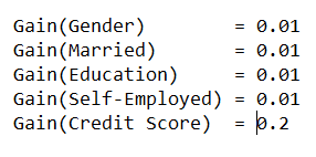
Credit Score has the highest gain so that will be used in the root node
Now let’s verify with the decision tree of the model.
Step 5: Visualize the Decision Tree
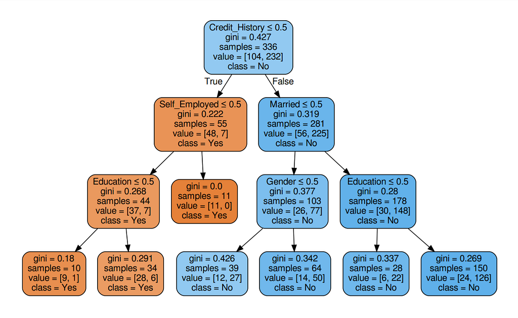
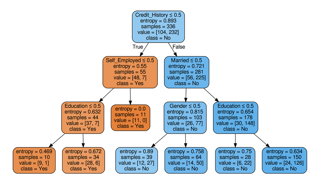
Well, it’s like we got the calculations right!
So the same procedure repeats until there is no possibility for further splitting.
Step 6: Check the score of the model
We almost got 80% percent accuracy. Which is a decent score for this type of problem statement?
Let’s get back with the theoretical information about the decision tree.
Assumptions made while creating the decision tree:
- While starting the training, the whole data-set is considered as the root.
- The input values are preferred to be categorical.
- Records are distributed based on attribute values.
- The attributes are placed as the root node of the tree is based on statistical results.
Optimizing the performance of the trees
- max_depth: The maximum depth of the tree is defined here.
- criterion: This parameter takes the criterion method as the value. The default value is Gini.
- splitter: This parameter allows us to choose the split strategy. Best and random are available types of the split. The default value is best.
Try changing the values of those variables and you will find some changes in the model’s accuracy.
How to avoid Over-Fitting?
Use Random Forest trees.
Advantages
- Decision trees are easy to visualize.
- Non-linear patterns in the data can be captures easily.
- It can be used for predicting missing values, suitable for feature engineering techniques.
Disadvantages
- Over-fitting of the data is possible.
- The small variation in the input data can result in a different decision tree. This can be reduced by using feature engineering techniques.
- We have to balance the data-set before training the model.
Conclusion
I hope everything is clear about decision trees. I tried to explain it easily. A clap and follow are appreciated.
Stay tuned for more.
Decision Trees Explained With a Practical Example was originally published in Towards AI — Multidisciplinary Science Journal on Medium, where people are continuing the conversation by highlighting and responding to this story.
Published via Towards AI
Related posts


Comments (3)
Leave a Reply to Alex Cancel reply
Popular posts

 for 2021")


Updates

Recent Posts


Alex
clap clap very nice
r
Clap clap 🙂
Eoin
Thanks You!