Want to Learn Quantization in The Large Language Model?

Author(s): Milan Tamang

Originally published on Towards AI.

Want to Learn Quantization in The Large Language Model?

Before I explain the diagram above, let me begin with the highlights that you’ll be learning in this post.

1. At first, you’ll learn about the what and why of the quantization.
2. Next, you’ll dive in further to learn the how of quantization with some simple mathematical derivations.
3. Finally, we’ll write some code together in PyTorch to perform quantization and de-quantization of LLM weight parameters

Let’s unpack all one by one together.

1. What is quantization and why do you need it?

Quantization is a method of compressing a larger size model (LLM or any deep learning model) to a smaller size. Primarily in quantization, you’ll quantize the weight parameters and activations of the model. Let’s do a simple model size calculation to validate our statement.

In the figure above, the size of the base model Llama 3 8B is 32 GB. After Int 8 quantization, the size is reduced to 8Gb (75% less). With Int4 quantization, the size has further reduced to 4GB (~90% less). This is a huge reduction in model size. And this is indeed amazing! isn’t it? Huge credit goes to the authors of quantization papers and my huge appreciation for the power of Mathematics.

Now that you understand what quantization is, let’s move on to the why part. Let’s look at image 1, as an aspiring AI researcher, developer or architect, if you would like to perform model fine-tuning on your datasets or inferencing, most likely you won’t be able to do so on your machine or mobile device due to memory and processor constraints. Probably, like me, you’ll also have an angry face like option 1b. This brings us to option 1a, where you can have a cloud provider providing you with all the resources you want and can easily do any task with any models you want. But it will cost you a lot of money. If you can afford it, great. But if you have a limited budget, the good news is you still have option 2 available. This is where you can perform quantization methods to reduce the model’s size and conveniently use it in your use cases. If you have done your quantization well, you will get more or less the same accuracy similar to that of the original model.

Note: Once you’ve done fine-tuning or other tasks on your model in your local machines if you want to bring your model into production, I would advise you to host your model in the cloud to offer reliable, scalable and secure services to your customer.

2. How does quantization work? A simple mathematical derivation.

Technically, quantization maps the model’s weight value from higher precision (eg. FP32) to lower precision (eg. FP16|BF16|INT8). Although there are many quantization methods available, in this post, we’ll learn one of the widely used quantization methods called the linear quantization method in this post. There are two modes in linear quantization: A. Asymmetric quantization and B. Symmetric quantization. We’ll learn about both methods one by one.

A. Asymmetric Linear Quantization: Asymmetric quantization method maps the values from the original tensor range (Wmin, Wmax) to the values in the quantized tensor range (Qmin, Qmax).

• Wmin, Wmax: Min and Max value of original tensor (data type: FP32, 32-bit floating point). The default data type of weight tensors in most modern LLM is FP32.
• Qmin, Qmax: Min and Max value of quantized tensor (data type: INT8, 8-bit integer). We can also choose other data types such as INT4, INT8, FP16, and BF16 for quantization. We’ll use INT 8 in our example.
• Scale value (S): During quantization, the scale value scales down the values of the original tensor to get a quantized tensor. During dequantization, it scales up the value of the quantized tensor to get de-quantized values. The data type of scale value is the same as the original tensor, which is FP32.
• Zero point (Z): The Zero point is the non-zero value in the quantized tensor range that directly gets mapped to the value 0 in the original tensor range. The data type of zero-point is INT8 since it is located in the quantized tensor range.
• Quantization: The “A” section of the diagram shows the quantization process which maps [Wmin, Wmax] -> [Qmin, Qmax].
• De-quantization: The “B” section of the diagram shows the de-quantization process which maps [Qmin, Qmax] -> [Wmin, Wmax].

So, how do we derive the quantized tensor value from the original tensor value? it’s quite simple. If you still remember your high-school mathematics, you can easily understand the derivation below. Let’s do it step by step (I suggest you refer to the diagram above while deriving your equation for more clear understanding).

I know many of you mightn’t want to go through the mathematical derivation below. But believe me, it will certainly help you to make your concept crystal clear and save you tons of time while coding for quantization in a later stage. I felt the same when I was researching this.

• Potential Issue 1: What to do if the value of Z runs out of the range? Solution: Use a simple if-else logic to change the value of Z to Qmin if it is smaller than Qmin and to Qmax if it is bigger than Qmax. This has been described well in Figure A of image 4 below.
• Potential Issue 2: What to do if the value of Q runs out of the range? Solution: In PyTorch, there is a function called clamp, which adjusts the value to remain within the specific range (-128, 127 in our example). Hence, the clamp function adjusts Q value to Qmin if it is below Qmin and to Qmax it is above Qmax. Problem solved, let’s move on.

Side note: The range of quantized tensor value is (-128, 127) for INT8, signed integer data type. If the data type of quantized tensor value is UINT8, unsigned integer, the range will be (0, 255).

B. Symmetric Linear Quantization: In the symmetric method, the 0 point in the original tensor range maps to the 0 point in the quantized tensor range. Hence, this is called symmetric. Since 0 is mapped to 0 on either side of the range, there is no Z (Zero Point) in symmetric quantization. The overall mapping happens between (-Wmax, Wmax) of the original tensor range to (-Qmax, Qmax) of the quantized tensor range. The diagram below shows the symmetric mapping in both quantized and de-quantized case.

Since we’ve defined all the parameters in asymmetric segment, the same applies here as well. Let’s get into the mathematical derivation of the symmetric quantization.

Difference between Asymmetric and Symmetric quantization:

Now that you have learned what, why, and how about linear quantization, this leads us to the final part of our post, the coding part.

3. Writing code in PyTorch to perform quantization and de-quantization of LLM weight parameters.

As I mentioned earlier, quantization can be done on the model’s weights, parameters, and activations as well. However, for simplicity, we’ll only quantify weight parameters in our coding example. Before we begin coding, let’s have a quick look at how weight parameter values change after quantization in the transformer model. I believe this will make our understanding further clearer.

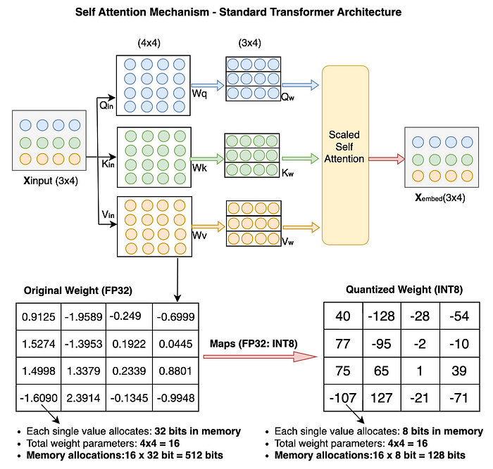
After we performed quantization on just 16 original weight parameters from FP32 to INT8, the memory footprint was reduced from 512 bits to 128 bits (25% reduction). This proves that for the case of large models, the reduction will be more significant.

Below, you can see the distribution of data types such as FP32, Signed INT8 and Unsigned UINT8 in actual memory. I’ve done the actual calculation in 2’s compliment. Feel free to practice calculation yourself and verify the results.

Now, that we’ve covered everything that you need to begin coding. I would suggest you follow along to get comfortable with the derivation.

A. Asymmetric quantization code: Let’s code step by step.

Step 1: We’ll first assign random values to the original weight tensor (size: 4×4, datatype: FP32)

# !pip install torch; install the torch library first if you've not yet done so
# import torch library 
import torch

original_weight = torch.randn((4,4))
print(original_weight)

Step 2: We’re going to define two functions, one for quantization and another for de-quantization.

def asymmetric_quantization(original_weight):
 # define the data type that you want to quantize. In our example, it's INT8.
 quantized_data_type = torch.int8

 # Get the Wmax and Wmin value from the orginal weight which is in FP32.
 Wmax = original_weight.max().item()
 Wmin = original_weight.min().item()
 
 # Get the Qmax and Qmin value from the quantized data type. 
 Qmax = torch.iinfo(quantized_data_type).max
 Qmin = torch.iinfo(quantized_data_type).min

 # Calculate the scale value using the scale formula. Datatype - FP32.
 # Please refer to math section of this post if you want to find out how the formula has been derived. 
 S = (Wmax - Wmin)/(Qmax - Qmin)

 # Calculate the zero point value using the zero point formula. Datatype - INT8.
 # Please refer to math section of this post if you want to find out how the formula has been derived.
 Z = Qmin - (Wmin/S)
 # Check if the Z value is out of range.
 if Z < Qmin:
 Z = Qmin
 elif Z > Qmax:
 Z = Qmax
 else:
 # Zero point datatype should be INT8 same as the Quantized value.
 Z = int(round(Z))

 # We have original_weight, scale and zero_point, now we can calculate the quantized weight using the formula we've derived in math section.
 quantized_weight = (original_weight/S) + Z

 # We'll also round it and also use the torch clamp function to ensure the quantized weight doesn't goes out of range and should remain within Qmin and Qmax.
 quantized_weight = torch.clamp(torch.round(quantized_weight), Qmin, Qmax)

 # finally cast the datatype to INT8.
 quantized_weight = quantized_weight.to(quantized_data_type)

 # return the final quantized weight.
 return quantized_weight, S, Z

def asymmetric_dequantization(quantized_weight, scale, zero_point):
 # Use the dequantization calculation formula derived in the math section of this post.
 # Also make sure to convert quantized_weight to float as substraction between two INT8 values (quantized_weight and zero_point) will give unwanted result. 
 dequantized_weight = scale * (quantized_weight.to(torch.float32) - zero_point)

 return dequantized_weight

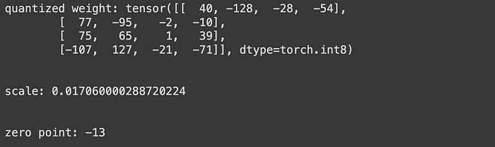
Step 3: We’re going to calculate the quantized weight, scale and zero point by invoking the asymmetric_quantization function. You can see the output result in the screenshot below, take note that the data type of quantized_weight is int8, scale is FP32 and zero_point is INT8.

quantized_weight, scale, zero_point = asymmetric_quantization(original_weight)
print(f"quantized weight: {quantized_weight}")
print("\n")
print(f"scale: {scale}")
print("\n")
print(f"zero point: {zero_point}")

Step 4: Now that we have all the values of quantized weight, scale and zero point. Let’s get the de-quantized weight value by invoking the asymmetric_dequantization function. Note that the de-quantize weight value is FP32.

dequantized_weight = asymmetric_dequantization(quantized_weight, scale, zero_point)
print(dequantized_weight)

Step 5: Let’s find out how accurate is the final de-quantized weight value as compared to the original weight tensor by calculating the quantization error between them.

quantization_error = (dequantized_weight - original_weight).square().mean()
print(quantization_error)

Output Result: The quantization_error is so much less. Hence, we can say that the asymmetric quantization method has done a great job.

B. Symmetric quantization code: We’re going to use the same code that we’ve written in the asymmetric method. The only change required in the case of the symmetric method is to always ensure the value of zero_input to be 0. This is because, in symmetric quantization, the zero_input value always maps to the 0 value in the original weight tensor. And we can just proceed without needing to write additional code.

And this is it! we’ve come to the end of this post. I hope this post has helped you build solid intuition on quantization and a clear understanding of the mathematical derivation part.

My final thoughts…

• In this post, we have covered all the necessary topics that is required for you to get involved in any LLM or deep learning quantization-related task.
• Although, we’ve successfully done quantization on weight tensor and also achieved good accuracy. This is sufficient enough in most of the cases. However, If you want to apply quantization on a larger model with more accuracy, you need to perform channel quantization (quantize each row or column of the weight matrix) or group quantization (make smaller groups in the row or column and quantize them separately). These techniques are more complicated. I will cover them in my upcoming post.

Stay tuned, and Thanks a lot for reading!

Link to Google Colab notebook

References

• From huggingface Blog: https://huggingface.co/docs/optimum/en/concept_guides/quantization#pratical-steps-to-follow-to-quantize-a-model-to-int8
• From huggingface blog: https://huggingface.co/blog/hf-bitsandbytes-integration

Join thousands of data leaders on the AI newsletter. Join over 80,000 subscribers and keep up to date with the latest developments in AI. From research to projects and ideas. If you are building an AI startup, an AI-related product, or a service, we invite you to consider becoming a sponsor.

Published via Towards AI