Unsupervised vs. Supervised Learning

Last Updated on August 24, 2020 by Editorial Team

Author(s): Rajaram VR

Machine Learning

I just started my initial steps into data science and machine learning, and, got introduced to “Supervised Learning” techniques as “Classifiers (Decisiontreeclassifer from sklearn kit), and on the unsupervised learning, with “Clustering.”

In this case, we are using the dataset “Breast cancer — Wisconsin” and set the following objective:

a) Perform clustering (k-means), use evaluation methods like silhouette score and WSS (within the sum of squares) to find optimal clusters,

b) Perform a Decisiontreeclassifier model, and the traditional train versus test samples and evaluate the model with ROC/AUC

c) Compare the clustering model output with the efficiency of Decisiontreeclassifer model outcome

The comparison outcome, presented a surprise to me, were without the target/class variables, the accuracy with just clustering, was close to 95 % match to the actual class variables in the data set, better than Supervised learning (with 70: 30, train to test split up, the accuracy was 92 % ). Now, does this mean it will work for larger samples also, is to be validated for larger data sets?

Let us get started — Data insights :

Features are a digitized image compilation of a fine needle aspirate (FNA) of a breast mass. They describe the characteristics of the cell nuclei present in the image.

Total rows — 569, columns — 32 (including class variable, called diagnosis, with the outcome as Malignant (M) and Benign (B).

The Data Process steps are:

The Data set did not have any missing or duplicate values, but had a lot of outliers, across most of the columns, and the treatment of outliers was an IQR based outlier treatment, which was followed by standardization (zScore) as the scale and range were different between features.

This cleansed data, was separated into features and classes (target) and then provided as input to both K-Means Clustering and also Decisiontreeclassifier models.

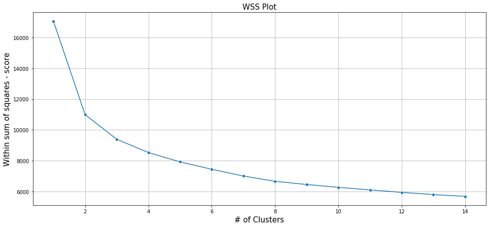
K-Means Clustering is an Un-supervised ML algorithm used to identify the number of clusters of target variables given a data set. Let us ignore the target variable in the original data set and look at only features. Let us assume there is no knowledge of potential clusters of the target variable. Given this data set, and looking at the WSS plot below, it might seem there is no significant change in the WSS score, from 8 onwards. So the number of clusters from this plot maybe like 8. But given the business scenario of “Cancer data set,” it wouldn’t make sense to have 8 class buckets or targets.

Further, validate this, let us look at the silhouette score.

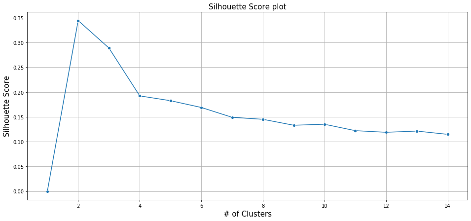
The silhouette score is a measure of the average distance between clusters and how tightly observations are clustered in a cluster. Though the WSS plot indicates an optimal cluster of 8, the silhouette score is more apt, as the optimal cluster is indicative of the “average score,” and the maximum average score as per above Silhouette score plot is at 2 clusters.

Supervised Learning — Decisiontreeclassifier

As the name suggests, a supervised learning model requires both features and the target variable (class variable), in this supervised learning approach, we are going to use a decision tree to classify rows based on features, into a binary decision outcome 1 or 0. In the business scenario considered, one would mean Malignant (M), and 0 would mean Benign (B).

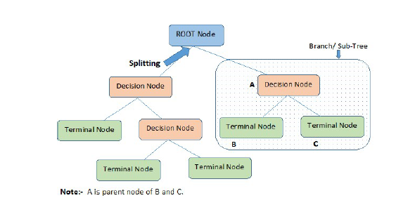
In this model approach, a decision tree, is constructed at the end, and it typically has the Root node, branch / sub-tree (under root nodes), as depicted below, the higher the number of branches, it would mean the model is overfitted, and fewer branches would mean underfitting. An optimal approach or number of branches is what would be required, and the evaluation mechanism of such models, are varied, and we would use confusion matrix and Area under curve AUC and ROC (Receiver operating characteristics) to validate the model efficiency. A decision tree is depicted below,

“Decisiontreeclassifier” modeling available under sklearn.tree module

dt_model = DecisionTreeClassifier(criterion = ‘gini’ ,random_state=123)

before invoking the model, and fitment, we split the data set into training and testing samples, using the sklearn. Model selection module and library train_test_split. We present a 70:30 split between train and test.

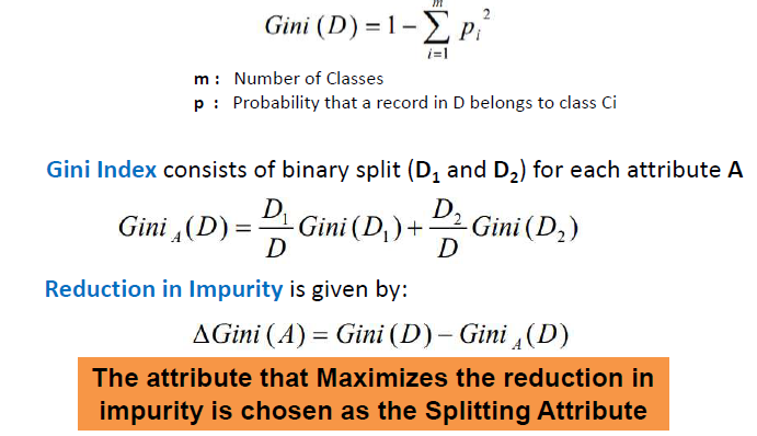
A quick glance at the parameters, we would be using “Gini” criteria, which is, basically,

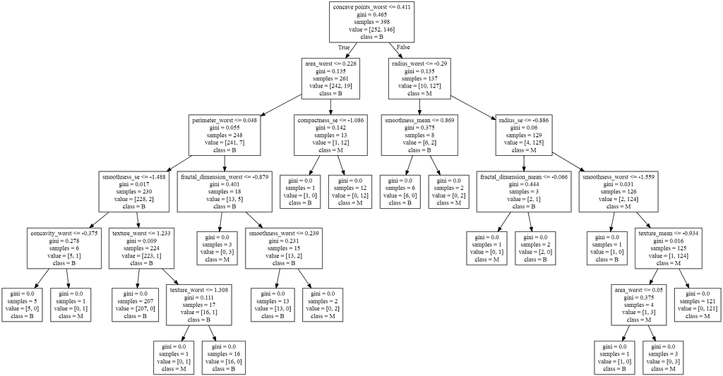
The decision tree, generated above, depicts six branches, for the training set, the decision tree classifier model, provides a “features_importance” for every feature. This is critical to understand how each feature influences the final outcome and what is the weight of each, the below plot depicts which features have stronger influences,

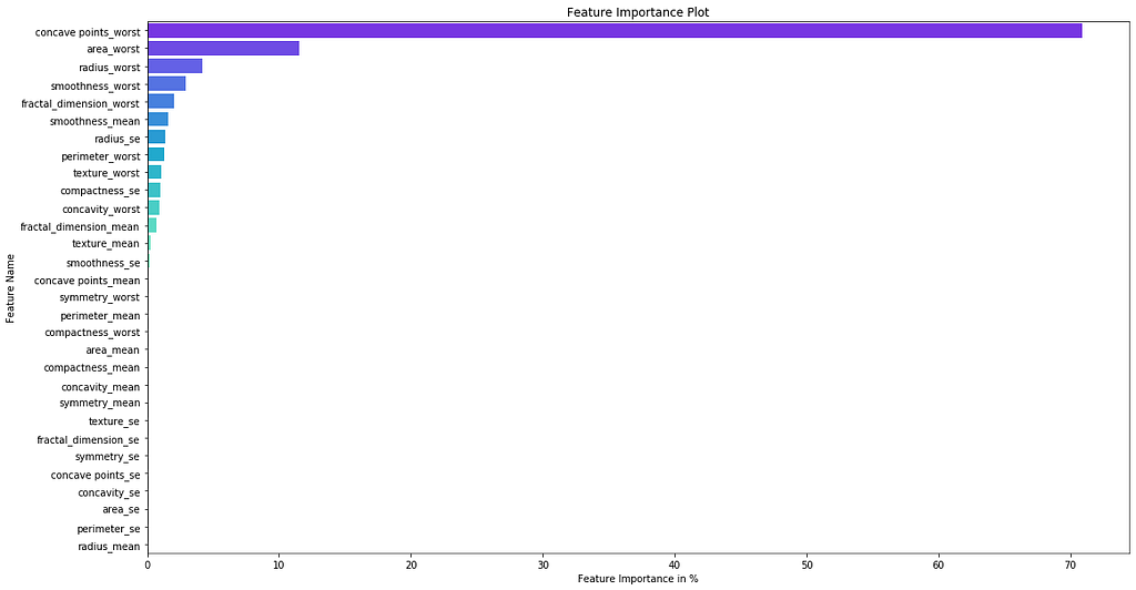
If we notice the feature, “Concave Points_worst” has the most substantial influence of 70.9%, and the root_node uses this feature to generate the split to the next branch basically.

Let us look at the AUC plots for training data set, test data set, and comparison of K-Means with test and training data set.

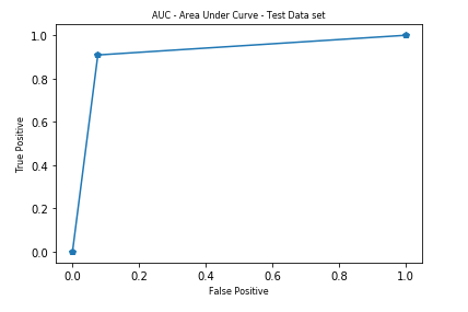
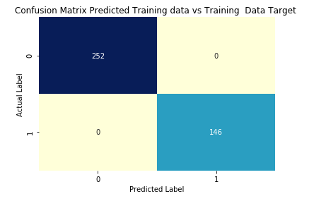
If you notice, the AUC is less for test data set, @ 0.916, while training data set was at 1, meaning the train labels when compared to the actual data set, class variables (diagnosis) were exactly matching.

When comparing the AUC between kMeans outcome and train, test respectively,

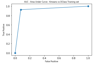
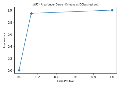
The AUC scores for the Kmeans outcome (only training samples) compared to the training data set, is 0.925, and for the testing dataset, it is 0.908.

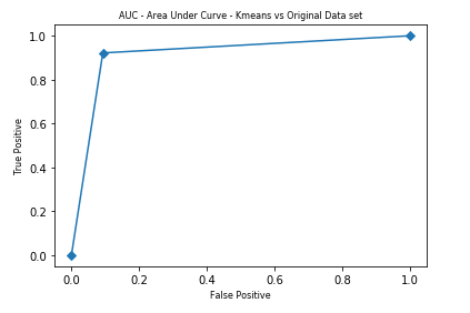
When comparing the kMeans score with original data (Diagnosis) class labels, the above AUC indicates high conformance between kMeans output and Diagnosis class (Benign — 0, Malignant — 1). The AUC score was also high at 0.915.

The following are the confusion matrix, for different scenarios,

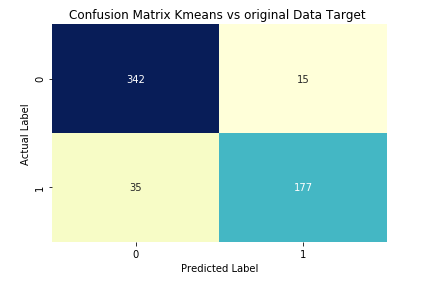
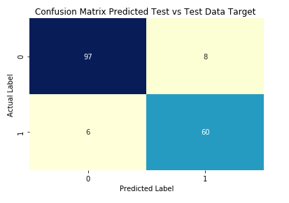
The consolidated final data, with a comparison between “Diagnosis” original target (class) variable, Kmeans clustering output, Training prediction, Test prediction, is available at

In conclusion, KMeans clustering provides similar accuracy and fit , even though it is un-supervised learning, when compared to Decisiontreeclassifier which is a supervised learning.

Unsupervised vs. Supervised Learning was originally published in Towards AI — Multidisciplinary Science Journal on Medium, where people are continuing the conversation by highlighting and responding to this story.

Published via Towards AI