


ResNet Architecture: Deep Learning with PyTorch
Last Updated on July 24, 2023 by Editorial Team
Author(s): Satyam Kumar Singh
Originally published on Towards AI.
Deep Learning
From winning ImageNet Large Scale Visual Recognition Challenge (ILSVRC) in 2015 till now ResNet Architecture has been remarkable in the field of Data Science. Apart from ILSVRC, ResNet also won Detection and localization challenge and MSCOCO detection and segmentation challenge. Quite a feat!
So, What’s so unique about ResNet compared to the previous convolutional network?
ResNet: the working behind it
As input=output, So effectively the more the layers the better the network. Well, not actually. But in the real world, because of the vanishing gradient and curse of dimensionality problems, it isn’t possible. In fact, the training error increases after certain epochs.
The working is ResNet is pretty simple, it adds the original input back to the output feature map obtained by passing the input through one or more convolutional layers.

Lets us understand the picture on the left. What’s happening is Relu(Input+Output), where input is either the 1st data or the data of previous block and output is Relu(W2(W1+b) + I), where W1 and W2 are the weight of both layers and b is the bias of the previous layer.
Now as we know the basic behind the ResNet architecture, so let’s create one.
class SimpleResidualBlock(nn.Module):
 def __init__(self):
 super().__init__()
 self.conv1 = nn.Conv2d(in_channels=3, out_channels=3, kernel_size=3, stride=1, padding=1)
 self.relu1 = nn.ReLU()
 self.conv2 = nn.Conv2d(in_channels=3, out_channels=3, kernel_size=3, stride=1, padding=1)
 self.relu2 = nn.ReLU()

 def forward(self, x):
 out = self.conv1(x)
 out = self.relu1(out)
 out = self.conv2(out)
 return self.relu2(out) + x # ReLU can be applied before or after adding the input
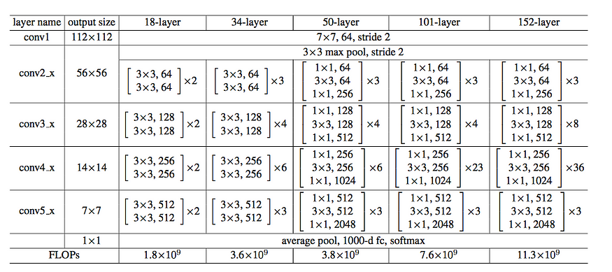
Note something above, if the dimensions of our output don’t match our residual then we cannot perform Relu addition, hence, we shall not only apply pooling on the input, but the residual would also be transformed through a stridden 1 x 1 conv that would project the filters to be the same as the output and the stride of 2 would half the dimensions just as the max-pooling does.

In the above picture, we saw ResNet34 architecture. The first layer with 7×7 convolution and stride 2 to down sample the input pooling it by the factor of 2. Then it’s followed by 3 identity blocks before down sampling again by 2. In the last average pooling layer, it creates 1000 feature maps, and average it for each feature map. The result is a 1000 dimensional vector which is then fed into the Softmax layer directly making him fully convolutional. There are a total of 6 different types of ResNet architectures namely, ResNet9, ResNet18, ResNet34, ResNet50, Resnet101, ResNet150 differing in the number of layers. After explaining all, I should now present the full ResNet.
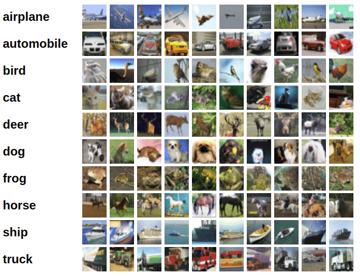
Classifying CIFAR10 images using ResNet and Regularization techniques in PyTorch
Here are some images from the dataset:
System Setup
# Uncomment and run the commands below if imports fail
# !conda install numpy pandas pytorch torchvision cpuonly -c pytorch -y
# !pip install matplotlib --upgrade --quiet
import os
import torch
import torchvision
import tarfile
import torch.nn as nn
import numpy as np
import torch.nn.functional as F
from torchvision.datasets.utils import download_url
from torchvision.datasets import ImageFolder
from torch.utils.data import DataLoader
import torchvision.transforms as tt
from torch.utils.data import random_split
from torchvision.utils import make_grid
import matplotlib.pyplot as plt
%matplotlib inlineproject_name='05b-cifar10-resnet'
Preparing the Data
Let’s begin by downloading the dataset and creating PyTorch datasets to load the data, just as we did in the previous tutorial.
# Dowload the dataset
dataset_url = "http://files.fast.ai/data/cifar10.tgz"
download_url(dataset_url, '.')

# Extract from archive
with tarfile.open('./cifar10.tgz', 'r:gz') as tar:
 tar.extractall(path='./data')

# Look into the data directory
data_dir = './data/cifar10'
print(os.listdir(data_dir))
classes = os.listdir(data_dir + "/train")
print(classes)# Data transforms (normalization & data augmentation)
stats = ((0.4914, 0.4822, 0.4465), (0.2023, 0.1994, 0.2010))
train_tfms = tt.Compose([tt.RandomCrop(32, padding=4, padding_mode='reflect'),
 tt.RandomHorizontalFlip(),
 tt.ToTensor(),
 tt.Normalize(*stats,inplace=True)])
valid_tfms = tt.Compose([tt.ToTensor(), tt.Normalize(*stats)])
# PyTorch datasets
train_ds = ImageFolder(data_dir+'/train', train_tfms)
valid_ds = ImageFolder(data_dir+'/test', valid_tfms)
batch_size = 400
# PyTorch data loaders
train_dl = DataLoader(train_ds, batch_size, shuffle=True, num_workers=3, pin_memory=True)
valid_dl = DataLoader(valid_ds, batch_size*2, num_workers=3, pin_memory=True)
def show_batch(dl):
 for images, labels in dl:
 fig, ax = plt.subplots(figsize=(12, 12))
 ax.set_xticks([]); ax.set_yticks([])
 ax.imshow(make_grid(images[:64], nrow=8).permute(1, 2, 0))
 break
show_batch(train_dl)

Using a GPU
def get_default_device():
 """Pick GPU if available, else CPU"""
 if torch.cuda.is_available():
 return torch.device('cuda')
 else:
 return torch.device('cpu')

def to_device(data, device):
 """Move tensor(s) to chosen device"""
 if isinstance(data, (list,tuple)):
 return [to_device(x, device) for x in data]
 return data.to(device, non_blocking=True)

class DeviceDataLoader():
 """Wrap a dataloader to move data to a device"""
 def __init__(self, dl, device):
 self.dl = dl
 self.device = device

 def __iter__(self):
 """Yield a batch of data after moving it to device"""
 for b in self.dl:
 yield to_device(b, self.device)

 def __len__(self):
 """Number of batches"""
 return len(self.dl)
train_dl = DeviceDataLoader(train_dl, device)
valid_dl = DeviceDataLoader(valid_dl, device)def accuracy(outputs, labels):
 _, preds = torch.max(outputs, dim=1)
 return torch.tensor(torch.sum(preds == labels).item() / len(preds))

class ImageClassificationBase(nn.Module):
 def training_step(self, batch):
 images, labels = batch
 out = self(images) # Generate predictions
 loss = F.cross_entropy(out, labels) # Calculate loss
 return loss

 def validation_step(self, batch):
 images, labels = batch
 out = self(images) # Generate predictions
 loss = F.cross_entropy(out, labels) # Calculate loss
 acc = accuracy(out, labels) # Calculate accuracy
 return {'val_loss': loss.detach(), 'val_acc': acc}

 def validation_epoch_end(self, outputs):
 batch_losses = [x['val_loss'] for x in outputs]
 epoch_loss = torch.stack(batch_losses).mean() # Combine losses
 batch_accs = [x['val_acc'] for x in outputs]
 epoch_acc = torch.stack(batch_accs).mean() # Combine accuracies
 return {'val_loss': epoch_loss.item(), 'val_acc': epoch_acc.item()}

 def epoch_end(self, epoch, result):
 print("Epoch [{}], last_lr: {:.5f}, train_loss: {:.4f}, val_loss: {:.4f}, val_acc: {:.4f}".format(
 epoch, result['lrs'][-1], result['train_loss'], result['val_loss'], result['val_acc']))def conv_block(in_channels, out_channels, pool=False):
 layers = [nn.Conv2d(in_channels, out_channels, kernel_size=3, padding=1),
 nn.BatchNorm2d(out_channels),
 nn.ReLU(inplace=True)]
 if pool: layers.append(nn.MaxPool2d(2))
 return nn.Sequential(*layers)

class ResNet9(ImageClassificationBase):
 def __init__(self, in_channels, num_classes):
 super().__init__()

 self.conv1 = conv_block(in_channels, 64)
 self.conv2 = conv_block(64, 128, pool=True)
 self.res1 = nn.Sequential(conv_block(128, 128), conv_block(128, 128))

 self.conv3 = conv_block(128, 256, pool=True)
 self.conv4 = conv_block(256, 512, pool=True)
 self.res2 = nn.Sequential(conv_block(512, 512), conv_block(512, 512))

 self.classifier = nn.Sequential(nn.MaxPool2d(4),
 nn.Flatten(),
 nn.Linear(512, num_classes))

 def forward(self, xb):
 out = self.conv1(xb)
 out = self.conv2(out)
 out = self.res1(out) + out
 out = self.conv3(out)
 out = self.conv4(out)
 out = self.res2(out) + out
 out = self.classifier(out)
 return out
model = to_device(ResNet9(3, 10), device)
model
Training the model
@torch.no_grad()
def evaluate(model, val_loader):
model.eval()
outputs = [model.validation_step(batch) for batch in val_loader]
return model.validation_epoch_end(outputs)
def get_lr(optimizer):
for param_group in optimizer.param_groups:
return param_group['lr']
def fit_one_cycle(epochs, max_lr, model, train_loader, val_loader,
weight_decay=0, grad_clip=None, opt_func=torch.optim.SGD):
torch.cuda.empty_cache()
history = []
# Set up cutom optimizer with weight decay
optimizer = opt_func(model.parameters(), max_lr, weight_decay=weight_decay)
# Set up one-cycle learning rate scheduler
sched = torch.optim.lr_scheduler.OneCycleLR(optimizer, max_lr, epochs=epochs,
steps_per_epoch=len(train_loader))
for epoch in range(epochs):
# Training Phase
model.train()
train_losses = []
lrs = []
for batch in train_loader:
loss = model.training_step(batch)
train_losses.append(loss)
loss.backward()
# Gradient clipping
if grad_clip:
nn.utils.clip_grad_value_(model.parameters(), grad_clip)
optimizer.step()
optimizer.zero_grad()
# Record & update learning rate
lrs.append(get_lr(optimizer))
sched.step()
# Validation phase
result = evaluate(model, val_loader)
result['train_loss'] = torch.stack(train_losses).mean().item()
result['lrs'] = lrs
model.epoch_end(epoch, result)
history.append(result)
return historyhistory = [evaluate(model, valid_dl)]
history
epochs = 8
max_lr = 0.01
grad_clip = 0.1
weight_decay = 1e-4
opt_func = torch.optim.Adam
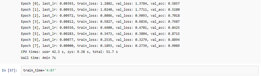
%%time
history += fit_one_cycle(epochs, max_lr, model, train_dl, valid_dl,
grad_clip=grad_clip,
weight_decay=weight_decay,
opt_func=opt_func)
def plot_accuracies(history):
accuracies = [x['val_acc'] for x in history]
plt.plot(accuracies, '-x')
plt.xlabel('epoch')
plt.ylabel('accuracy')
plt.title('Accuracy vs. No. of epochs');
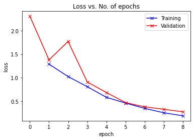
plot_accuracies(history)def plot_losses(history):
train_losses = [x.get('train_loss') for x in history]
val_losses = [x['val_loss'] for x in history]
plt.plot(train_losses, '-bx')
plt.plot(val_losses, '-rx')
plt.xlabel('epoch')
plt.ylabel('loss')
plt.legend(['Training', 'Validation'])
plt.title('Loss vs. No. of epochs');
plot_losses(history)def plot_lrs(history):
lrs = np.concatenate([x.get('lrs', []) for x in history])
plt.plot(lrs)
plt.xlabel('Batch no.')
plt.ylabel('Learning rate')
plt.title('Learning Rate vs. Batch no.');
plot_lrs(history)


Congratulations, for reaching this far. I know there is a lot of learning there but trust me this topic is worth reading.
Now, for further reading here are some awesome links that you should check.
Hope you loved this, future posts will be on GANs in deep learning.
Have a great time ahead!
You can always reach me on twitter and GitHub via @satyamkumar073.
Join thousands of data leaders on the AI newsletter. Join over 80,000 subscribers and keep up to date with the latest developments in AI. From research to projects and ideas. If you are building an AI startup, an AI-related product, or a service, we invite you to consider becoming a sponsor.
Published via Towards AI
Related posts


Popular posts

 for 2021")


Updates

Recent Posts


