


Practical Nuances of Time Series Forecasting — Part II— Improving Forecast Accuracy
Last Updated on January 5, 2024 by Editorial Team
Author(s): Santoshkumarpuvvada
Originally published on Towards AI.
Practical Nuances of Time Series Forecasting — Part II— Improving Forecast Accuracy
In continuation of enhancing our understanding of time series forecasting, let’s get started with part 2. (Check out the part 1 here). Many times, practitioners feel that they have done everything possible to achieve a good forecast estimate — capturing all available relevant data , proper data cleaning, applying all possible algorithms, and fine-tuning the algorithms & still, results sometimes may not be up to mark! Now, what if I told you there could be some simple yet efficient ways to bump up your accuracy by a few points? We are presenting you a popular technique — the Hybrid Forecasting Model!
Hybrid Forecasting Model:
The basic premise of hybrid forecasting is to combine the strengths of complementary algorithms & overcome the weaknesses of individual algorithms.
For example, the ETS family(or exponential smoothening family) of models excels at detecting trend & seasonality. However, they can’t include any external factors information like promotions or weather or holiday information, etc. Similarly, tree-based models like XG boost/ Random forest regressors excel at determining complicated relationships between dependent & independent variables but fail to detect the trend in data as they try to fit the forecast to a range of values seen in training data. Now, what if we can combine the best of both models? That will likely perform much better than individual models.
Let’s see a demo on how the hybrid model works using the famous airplane passengers data set & then you will get a clear understanding of Hybrid forecasts.
A brief on the data set: The dataset contains 3 columns — Date, Volume of Passengers and Promotion. The dataset indicates 12 years monthly volume of passengers from Jan 1949 to Dec 1960

Let’s plot the data before we go for the analysis.

There are a few missing values. Since there is a trend in data as per the graph, replacing the null values with Zero or by average value will not make much sense as they won’t reflect the underlying data pattern.
Still, let us see how data will look like when we replace missing values by mean (mean imputation)

Let us also see what happens when missing values are replaced by zeros.

Note that, unlike in machine learning where there is a feasibility to just drop the records with missing values, we can’t do that in time series data. Because time series data is an ordered data(ordered by date) where as order doesn't matter in a typical ML problem.
So, the best method to deal with missing values in this case would be a linear interpolation of data.

Train-Test Spilt : Since we have 12 years data, let us use first 10 years for training & last 2 years for evaluating the model performance.
train_len = 120
train = df[0:train_len] # Taking first 120 months as training set
test = df[train_len:] # Taking last 24 months as out-of-time test set
y_hat_hwa = test.copy() # y_hat_hwa is a data frame which is copy of test set
# i intend to use it for storing forecast from holt winter additive model(hwa)
Model 1 – Holt Winter Model (ETS family based model):
As data contains clear trend & seasonality based on the graph, we can use Holt Winter model for forecasting the volume of passengers. (Note: I will use the ETS model/Holt Winter/exponential smoothening interchangeably in the article, although they are not exactly the same. Refer to Appendix for further explanation)
model = ExponentialSmoothing(np.asarray(train['Volume']),seasonal_periods=12 ,trend='add',
 seasonal='add')
model_fit = model.fit(optimized=True)
print(model_fit.params)
y_hat_hwa['hw_forecast'] = model_fit.forecast(24)
# Since it is a monthly data , seasonal_periods is set to 12, if it is a quarterly data ,
# it could have been set as 4
# We are using an additive trend, additive seasonality in the above model

train['ETS fit'] = model_fit.fittedvalues
# Noting the ETS fitted values on the training data

# Plotting Actuals Vs ETS Forecast
plt.plot(y_hat_hwa['hw_forecast'], label = 'ETS forecast values')
plt.plot(test['Volume'],label= ' Test actuals')
plt.plot(train['Volume'],label= ' Train actuals')
plt.plot()
plt.legend()
plt.show()

# Calculate RMSE & MAPE of Holt winter forecast
rmse = np.sqrt(mean_squared_error(test['Volume'], y_hat_hwa['hw_forecast'])).round(2)
mape = np.round(np.mean(np.abs(test['Volume']-y_hat_hwa['hw_forecast'])/test['Volume'])*100,2)

tempResults = pd.DataFrame({'Method':['Holt Winters\' additive method'], 'RMSE': [rmse],'MAPE': [mape] })
results = pd.DataFrame()
results = pd.concat([results, tempResults])
results = results[['Method', 'RMSE', 'MAPE']]
results
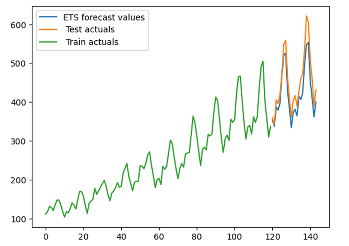
Following is the actuals Vs ETS forecast & below is the RMSE, MAPE of the ETS model

ETS forecast Vs Actuals in Test Period:
Let's have a closer look at actuals Vs. ETS forecast in the test period.
plt.plot(y_hat_hwa['hw_forecast'], label = 'ETS forecast values')
plt.plot(test['Volume'],label= 'actuals')
# Adding 'Promo' values with different markers
plt.plot(test.index[test['Promo'] == 1], test.loc[test['Promo'] == 1, 'Volume'], 'ro', label='Promo = 1') # 'ro' means red circles
plt.legend()
plt.show()

As we can see from the above graph, ETS is failing to capture the uplift that typically happens during promotions. This is expected as ETS model cant take external factors into consideration
Model 2 – XG Boost Regression:
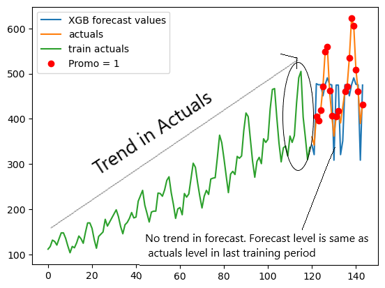
XG Boost is a popular & go-to ML algorithm for many tasks for practitioners. It can easily understand complex relations between dependent(y) & independent(x) variables. However, XG Boost has certain limitations in time series forecasting( like the inability to extend trend in the forecast). Let’s see how it performs on this data set
# We need to do feature engineering to apply XG boost(or any ML algorithm)
# for applying to time series forecasting as ML algorithms cant understand
# date as an input. I have done below simple feature engineering as it is just
# for a demo. More features can be added as per requirement

df['Month'] = df['Date'].dt.month
df['year'] = df['Date'].dt.year
df['Sr no.'] =df.index
Now, we can drop the date column as all useful information from date has been extracted. Month column should not be considered as a continuous variable but as a categorical variable. Hence, we add dummy variables for the same.
# Creating dummy variables for Month as follows:
train_Xgboost['Month'].replace({1:'Jan',2:'Feb',3:'March',4:'April',5:'May',6:'June',7:'July', 8:'Aug',9:'Sept', 10:'Oct', 11:'Nov', 12:'Dec'},inplace = True)
test_XGboost['Month'].replace({1:'Jan',2:'Feb',3:'March',4:'April',5:'May',6:'June',7:'July', 8:'Aug',9:'Sept', 10:'Oct', 11:'Nov', 12:'Dec'},inplace = True)
Months_train = pd.get_dummies(train_Xgboost['Month'], drop_first = True)
Months_test= pd.get_dummies(test_XGboost['Month'],drop_first = True)
train_Xgboost = pd.concat([train_Xgboost,Months_train], axis = 1)
test_XGboost = pd.concat([test_XGboost,Months_test],axis = 1)

# Dropping the Month column as dummy variables have already been created.
train_Xgboost_X.drop("Month",axis =1, inplace = True)
test_Xgboost_X.drop("Month",axis =1, inplace = True)

# Dropping the Volume from X Data Sets of train & Test
train_Xgboost_X = train_Xgboost.drop("Volume",axis =1)
test_Xgboost_X = test_XGboost.drop("Volume",axis =1)

# Creating the Y Datasets of train & Test
train_Xgboost_y = train_Xgboost['Volume']
test_Xgboost_y = test_XGboost['Volume']

# Creating an instance of XG Boost Regressor
reg = xgb.XGBRegressor(n_estimators = 1000, max_depth = 6, learning_rate = 0.01, verbose = True)
# Training of Xgboost Model
reg.fit(X = train_Xgboost_X,y= train_Xgboost_y)

# Predicting using the trained model of Xgboost Model
y_hat_XGBoost = test.copy()
y_hat_XGBoost['Xgboost forecast'] = reg.predict(X = test_Xgboost_X)

# Visualizing actuals vs XGB forecast
plt.plot(y_hat_XGBoost['Xgboost forecast'], label = 'XGB forecast values')
plt.plot(test['Volume'],label= 'actuals')
plt.plot(train['Volume'],label ='train actuals')

# Adding 'Promo' values with different markers
plt.plot(test.index[test['Promo'] == 1], test.loc[test['Promo'] == 1, 'Volume'], 'ro', label='Promo = 1') # 'ro' means red circles
plt.legend()
plt.show()

Model 3 — Hybrid Model( ETS + XG boost):
Now, let’s explore the implementation of Hybrid model & understand how it works.
Any time series can be expressed as a function of trend, seasonality, cyclicity, external regressors impact & error.
Some models may capture trend & seasonality better, as we saw with ETS, and some can capture external regressors' impact, like XG boost. So, the idea is to split time series into multiple parts & run different models on different parts. For example, when we subtract ETS Fitted data from the original training data, we get all the information that ETS couldn't learn/understand. This time series obtained by subtracting the fitted line(obtained by one forecast method) from the original time series is called residual time series.
train['Residual'] = train['Volume'] - train['ETS fit']
plt.plot(train['Volume'], label = 'Original Train data')
plt.plot(train['ETS fit'], label = 'ETS fitted data')
plt.plot(train['Residual'],label = "Difference of original data & fitted data")
plt.legend()
plt.show()

Now, assuming there is no overfitting in the 1st forecast method (ETS), the orange line/ ETS fitted data represents all the information it learned from the data & the green line/residual data contains information like Promo impact information and any other information + error which model was not able to learn.
Now, we can run an XG boost model on this green line. However, unlike in model 2 , where we passed information like month/year/Sr no. etc. we can now pass only promotion information for training as trend & seasonality were already taken care of by ETS.
# Preparing Training Data y for XGboost in the hybrid model
train_Xgboost_X_residual = train_Xgboost_X['Promo']
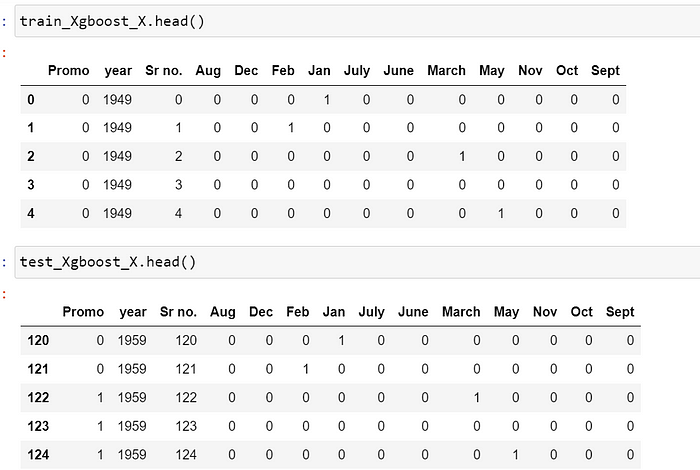
Training Data X & Training Data y looks like the following for XG Boost in the Hybrid Model:


# Training & prediction on Residual time series as Y & promo data as X using
# XG Boost
reg.fit(X = train_Xgboost_X_residual,y= train['Residual'])
Xgboost_prediction_on_residuals = reg.predict(X = test_Xgboost_X['Promo'])

#Combining the ETS Forecast & XG Boost forecast made using residual time series
y_hat_hwa['new'] = y_hat_hwa['hw_forecast']+Xgboost_prediction_on_residuals

# Calucating error of the New Hybrid forecast
# (ETS Forecast) +(XG boost forecast for the residual time series)
rmse = np.sqrt(mean_squared_error(test['Volume'], y_hat_hwa['new'])).round(2)
mape = np.round(np.mean(np.abs(test['Volume']-y_hat_hwa['new'])/test['Volume'])*100,2)

tempResults = pd.DataFrame({'Method':['Hybrid'], 'RMSE': [rmse],'MAPE': [mape] })
results = pd.concat([results, tempResults])

results = results[['Method', 'RMSE', 'MAPE']]
results

Hurray! The hybrid model performed better than both individual models!
# Visualizing Hybrid Forecast Vs Test Data Actuals
plt.plot(y_hat_hwa['new'], label = 'Hybrid')
plt.plot(test['Volume'],label= 'actuals')
# Adding 'Promo' values with different markers
plt.plot(test.index[test['Promo'] == 1], test.loc[test['Promo'] == 1, 'Volume'], 'ro', label='Promo = 1') # 'ro' means red circles
plt.legend()
plt.show()
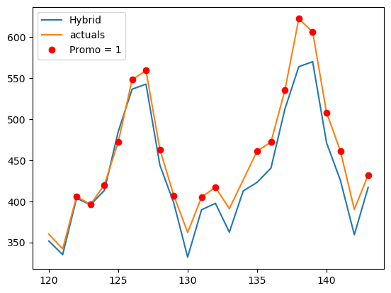
Now, it is clear that the hybrid model has outperformed both the individual models. The questions that can come to your mind are
- What if I create a hybrid forecast of 3 or more models? Will it be better than a hybrid of 2 forecast models?
Ans) Empirically, it has been found that a hybrid of 2 models is more than sufficient & there is no real added advantage as we keep on increasing the models other than increasing the complexity in implementation. Hence, stick to a hybrid of 2 models
2. What are models I can combine? Here, you used ETS + XG boost. What if I have weekly data where ETS won’t work?
Ans) Although there is no strict list that you can combine only these models, the basic premise is that models that will be used in hybrid forecast are complementary & suit the data at problem.
Some famous combinations that have worked well in previous time series competitions are as follows:
- STL + Exponential Smoothening
- Exponential Smoothening + LSTM neural network
- ARIMA + Boosted GBTs(Gradient-boosted decision trees)
So, that's a wrap about hybrid forecasting & part II of the series. There is still one more technique that can be used for effective forecast improvement & I will discuss that idea in the final & 3rd part of this series. Stay tuned! U+1F600
Appendix:
Holt Winter Vs Exponential Smoothening Family Vs ETS models:
Holt Winter is a part of the exponential smoothening family. ETS models and exponential smoothing models produce the same point forecasts. However, ETS models can also generate prediction intervals, which can’t be done using exponential smoothening models.
References:
- Airline passenger data set with promotions (https://drive.google.com/file/d/11A_bKLKyROSCizwG90ykOJirFCML3SXM/view?usp=sharing)
- Kaggle Time Series Course by Ryan Hol Brook (https://www.kaggle.com/code/ryanholbrook/hybrid-models )
- Python workbook for Hybrid Model demonstration(https://drive.google.com/file/d/11cGOHAnI3m3hbDPcBexg5_uW688nIlLp/view?usp=sharing)
- An image of cat lifting weights was generated using Canva ( https://www.canva.com/your-apps)
Join thousands of data leaders on the AI newsletter. Join over 80,000 subscribers and keep up to date with the latest developments in AI. From research to projects and ideas. If you are building an AI startup, an AI-related product, or a service, we invite you to consider becoming a sponsor.
Published via Towards AI
Towards AI Academy
We Build Enterprise-Grade AI. We'll Teach You to Master It Too.
15 engineers. 100,000+ students. Towards AI Academy teaches what actually survives production.
Start free — no commitment:
→ 6-Day Agentic AI Engineering Email Guide — one practical lesson per day
→ Agents Architecture Cheatsheet — 3 years of architecture decisions in 6 pages
Our courses:
→ AI Engineering Certification — 90+ lessons from project selection to deployed product. The most comprehensive practical LLM course out there.
→ Agent Engineering Course — Hands on with production agent architectures, memory, routing, and eval frameworks — built from real enterprise engagements.
→ AI for Work — Understand, evaluate, and apply AI for complex work tasks.
Note: Article content contains the views of the contributing authors and not Towards AI.
Related posts
Recent Posts


")


