Mastering Derivatives for Machine Learning

Author(s): Towards AI Editorial Team

Originally published on Towards AI.

Understanding the building blocks of machine learning

Photo by Michael Dziedzic on Unsplash

Author(s): Pratik Shukla

“Education is the movement from darkness to light” — Allan Bloom

Table of Contents:

1. The Slope of a straight line
2. The rise of derivatives
3. Definition of derivative
4. Using the definition of derivative
5. The First Derivative Test
6. Working Example of the First Derivative Test
7. The Second Derivative Test
8. The Inflection Point
9. Working Example of the Second Derivative Test
10. Checking for Inflection Point
11. Working Example when f’’(X)=0, and X is an Inflection Point
12. Why do we need the First Derivative Test?
13. Working Example when f’’(X)=0, and X is not an Inflection Point
14. Flowchart for the First Derivative Test
15. Flowchart for the Second Derivative Test
16. Flowchart for the Inflection Point Test
17. Resources and References

If you’re interested in machine learning, it’s likely that you’ve come across the term “derivative” before. Derivatives are a fundamental concept in calculus, and they play a crucial role in many machine-learning algorithms. Put simply, a derivative measures the rate of change of a function at a particular point. This information can be used to optimize functions, find local minima and maxima, and more. In this blog, we’ll dive into the world of derivatives and explore some of the key concepts that are relevant to machine learning. Specifically, we’ll focus on the first derivative test, the second derivative test, and the inflection test — all powerful tools for analyzing the behavior of a function at different points. By the end of this blog, you’ll have a solid understanding of how these tests work and how they can be used to improve your machine-learning models.

The Slope of a Straight Line:

A slope is something that helps us measure the rate of change of a line. The slope of a straight line can be positive, negative, zero, or undefined.

We all know that the slope of a straight line is given by the ratio of change in y to change in x. In other words, we can also say that the slope of a straight line is given by the rise over the run. Note that the slope of a straight line is always constant. We can put it into the mathematical form using the following formula.

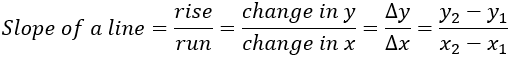Figure — 1: Equation of the slope of a straight line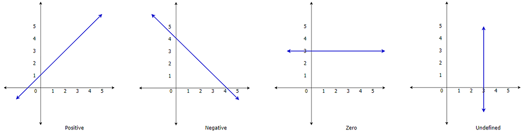Figure — 2: Slope of a straight line

The Rise of Derivatives:

In the 17th century, Isaac Newton and Gottfried Leibniz thought that the concept of slope can be applied to curves as well. They thought that instead of having a constant rate of change, we’ll have a variable rate of change in the case of curves. This is how the method of calculating the derivatives was born. Now, let’s see how this method works.

1. Step — 1:

In the below image, let’s say we want to find the slope at point P. To find the slope at point P, we will need to find the slope of the tangent line at point P.

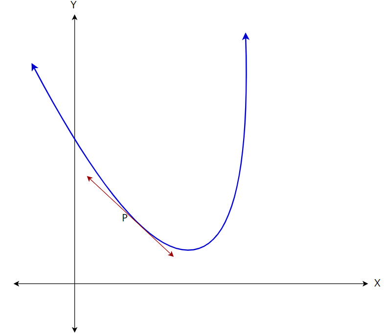Figure — 3: Finding the slope of the curve at point P

2. Step — 2:

But, as of now we only know how to find the slope of a straight line. To do that, let’s find another point on the curve and calculate the slope of the line between these two points.

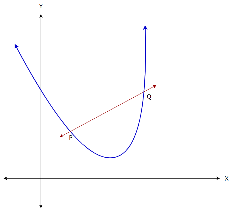Figure — 4: Finding the slope of the straight line PQ

3. Step — 3:

But here we can see that the above line does not represent the slope exactly at point P. Now, to find the slope exactly at point P, let’s find another point on the curve which is closer to P.

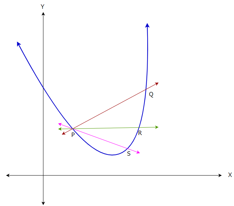Figure — 5: Finding more straight lines on the curve

4. Step — 4:

From the above image we can say that as we move the second point closer and closer, we are approaching our goal of finding the tangent line to point P. So, based on that, we can say that we just need to minimize the distance between the two points and keep it as close as 0. Let’s see how calculus can help us with this.

Let’s say the distance between the two points, P and Q is h. Now, our goal is to minimize the distance and keep it as close as 0. Here, we will use the concept of limits.

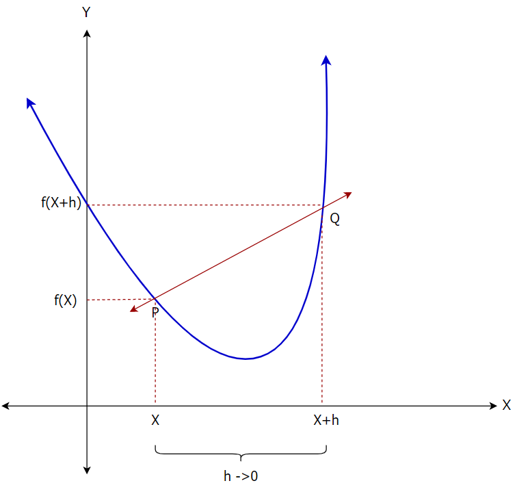Figure — 6: Finding the slope of the straight line PQ

Definition of Derivatives:

Derivatives are the essence of calculus. Basically, derivatives represent the instantaneous rate of change of a function with respect to one of its variables. Geometrically, a derivative is the slope of a tangent line of a curve at a point which signifies the rate of change at a particular point.

Mathematical Definition of Derivative:

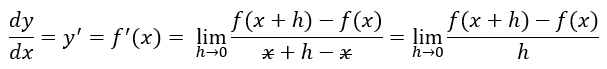Figure — 7: Mathematical definition of derivative

Using the Definition of Derivative:

Now, we know that we can find the derivative of any function using the following formula.

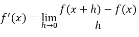Figure — 8: Mathematical Definition of Derivatives

Let’s take an example to understand how we can actually find the derivative using the above-given formula.

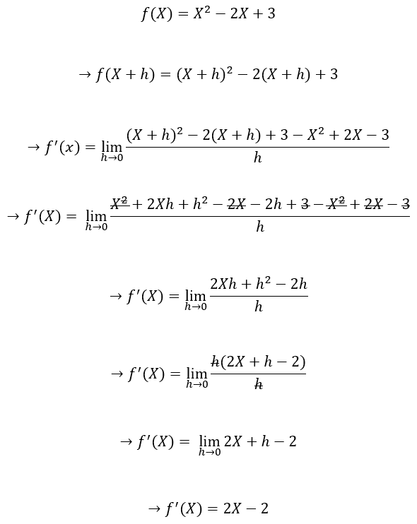Figure — 9: Calculating Derivatives Using the Mathematical Definition of Derivatives

The First Derivative Test:

We use the first derivative test to check whether a function is increasing or decreasing in its domain. We can also use this test to identify its local maxima and minima.

The first derivative of a function is the slope of the tangent line to the graph of a function at a given point. We can think of the first derivative as the slope of the function. When the slope is positive, the graph is increasing. When the slope is negative, the graph is decreasing. When the slope is 0, those points will be local maxima or minima. These points are called critical points. The first derivative test involves testing the behavior of the function around these points to determine whether or not they are local maxima or minima.

The first derivative test is based on the fact that the sign of the first derivative does not change between critical points. Thus, if we find the critical points of a function, we can test points within the intervals between critical points to determine whether the function is increasing or decreasing over those intervals. Then, by determining whether the function is increasing or decreasing before and after a critical point, we can identify whether the point is a minimum, maximum, or neither.

Let’s say we have a function f(X) which is plotted in the below image.

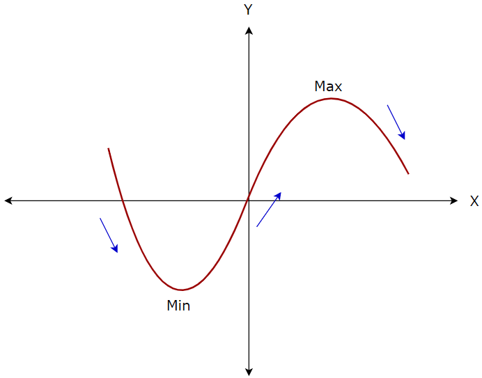Figure — 10: A Graph Showing Maximum and Minimum Points

Now, we can say the following things about the function.

1. Function f has a relative minimum at x=m if for all the points p near m, f(m)<f(p).
2. Function f has a relative maximum at x=m if for all the points p near m, f(m)>f(p).

The First Derivative Test:

Let’s say f is a differentiable function with f’(m) = 0. Based on this, we can derive the following conclusions.

1. If f’(x) changes from positive to negative at x=m, then f has a local maximum at m.
2. If f’(x) changes from negative to positive at x=m, then f has a local minimum at m.

Working Example of the First Derivative Test

Example: Find the relative extrema for f(X) = 2X³ — 3X² — 12X.

1. Step — 1:

Our function f(X) is given by…

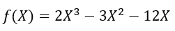Figure — 11: Function f(X)

2. Step — 2:

To find the relative extrema, we need to find the point(s) where the function's first derivative is 0.

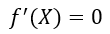Figure — 12: Finding the Critical Points of the Function f(X)

3. Step — 3:

Finding the points where the first derivative of the function (f’(X)) is 0.

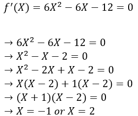Figure — 13: Finding Points Where f’(X)=0

4. Step — 4:

Now, we have two points where we will have relative maxima or minima. To find whether we have minima or maxima, we will need to check the points around these critical points. To do that, let’s find the intervals around these critical points.

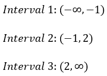Figure — 14: Finding Intervals based on the Critical Points

5. Step — 5:

Next, we will choose a point from each of the intervals and find the value of f’(X) for that chosen point. Here we will also note the sign of f’(X) for the chosen value of X in each interval. If the sign of f’(X) is positive (+), then it means that the function is increasing in that interval. On the other hand, if the sign of f’(X) is negative (-), then it means that the function is increasing in that interval.

The following table shows the required calculations.

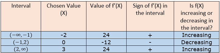Figure — 15: Calculating Whether f(X) is Increasing or Decreasing in the Intervals

6. Step — 6:

Based on the above table, we can say that we will have local maxima at point X = -1 as the value of f’(X) changes from positive to negative around it. On the other hand, we will have local minima at point X=2 as the value of f’(X) changes from negative to positive around it. Please note that the function does not change its value from positive to negative or negative to positive anywhere other than these critical points.

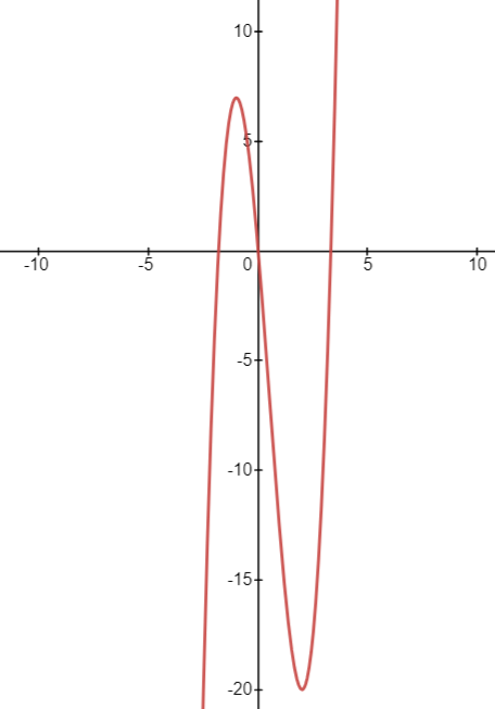Figure — 16: The Graph of the Function f(X)= 2X³-3X²-12X

The Second Derivative Test

We use the second derivative test to determine whether a critical point(s) of a function is a local minimum or maximum. We know that the first derivative is defined as the rate of change of the function, and it’s given by the slope of the tangential line at a given point on the curve. In the same way, the second derivative is the rate of change of the first derivative, and it’s also known as the concavity of f(X).

Before we dive into the second derivative test, let’s first understand the meaning of an inflection point.

The Inflection Point:

An inflection point is defined as a point on a curve at which the sign of the concavity changes. Inflection points cannot be local maxima or local minima. In the following image, we can see that for the function f(X) = X³, X = 0 is an inflection point. Also, we can see that in the interval (-inf,0), the function is concave and, in the interval, (0, inf), the function is convex.

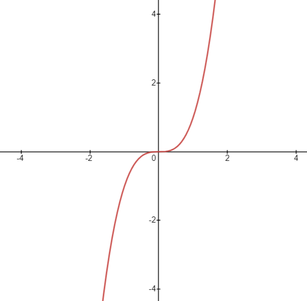Figure — 17: An Inflection Point

The Second Derivative Test:

Let’s say f(X) is a function such that f’(X) and f’’(X) can be defined for this function. Now, we can find all the critical points at f’(X) = 0. Next, we need to find the second derivative of the function at the critical points. The second derivative test is defined as follows:

• If f’’(X) > 0, then f(X) has a local minimum at X.
• If f’’(X)<0, then f(X) has a local maximum at X.
• If f’’(X) = 0, then we can say that the test is inconclusive. Now, it is possible that the point is an inflection point if the sign of f’’(X) changes from negative to positive or positive to negative around this point. But, if the sign of f’’(X) does not change, we can say that it is not an inflection point.

Steps Involved in Finding the Second Derivative:

1. We have the function f(X).
2. Find the critical points of the function by finding the points where the first derivative f’(X)=0.
3. Find the second derivative of the function f(X) at all the critical points.
4. If f’’(X)>0, then f(X) has a local minimum at X, and f(X) is a convex function in that interval.
5. If f’’(X)<0, then f(X) has a local maximum at X, and f(X) is a concave function in that interval.
6. If f’’(X)=0, then the second derivative test is inconclusive.
7. Check for inflection points.

Working Example of the Second Derivative Test

Example: Find the relative extrema for f(X) = 5X³ — 3X⁵

1. Step — 1:

Our function f(X) is given by…

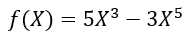Figure — 18: Function f(x)

2. Step — 2:

To find the relative extrema(s), we need to find the critical points. Critical points are the points where the first derivative of the function f’(X) = 0.

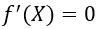Figure — 19: Finding the Critical Points of the Function f(X)

3. Step — 3:

Finding the points where the first derivative of the function (f’(X)) is 0.

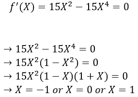Figure — 20: Finding Points Where f’(X)=0

4. Step — 4:

Now, we have three points where we might have relative maxima or minima. Next, we will find the second derivative f’’(X) of the function f(X) at these critical points.

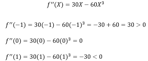Figure — 21: Finding the Second derivative

So, according to the second derivative test, we can say that we will have a local minimum at x=-1 and a local maximum at x=1.

5. Step — 5:

Now, we know that at X=0, the test is inconclusive. So, now let’s find whether X=0 is an inflection point or not. To do that, we need to test the concavity of f(X) before and after the inflection point by selecting a point from an appropriate interval. Here we know that the critical points are -1, 0, and 1. So, we need to choose a value from (-1,0) and (0,1). Let’s choose X=-0.5 and X=0.5 and see how it goes.

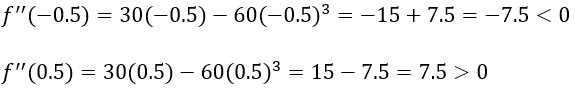Figure — 22: Finding an inflection point

Here, we can see that f’’(X) changes the sign around the point 0. So, we can say that 0 is an inflection point. Other than that, based on the results, we can say that the function is concave in the interval (-1,0) and convex in the interval (0,1).

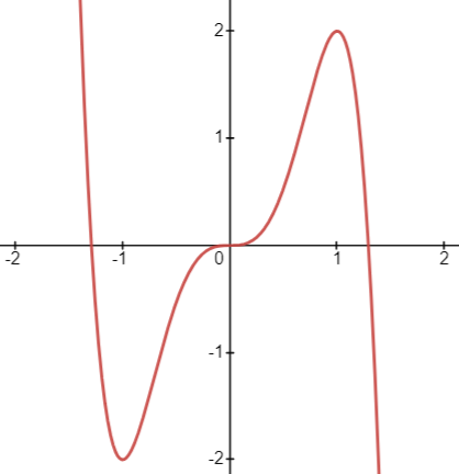Figure — 23: Monitoring the graph

Confusing Terms:

• Concave Up = Convex
• Concave Down = Concave

Checking for Inflection Point:

If f’’(X) =0 then there are two possibilities.

1. X is an inflection point — — End of the story
2. X is not an inflection point — — The story continues

Steps to check whether a critical point is an inflection point or not?

1. We know that f’’(X)=0.
2. Find appropriate intervals around critical point X.
3. Find the values of f’’(X) in these intervals.
4. If the sign of f’’(X) changes from negative (-) to positive (+) or positive (+) to negative (-) then it is an inflection point. If the f’’(X) sign does not change in these intervals, then it is not an inflection point.

Working Example when f’’(X)=0, and X is an Inflection Point:

1. Step — 1:

Our function f(X) is given by…

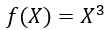Figure — 24: Function f(x)

2. Step — 2:

To find the relative extrema(s), we need to find the critical points. Critical points are the points where the first derivative of the function f’(X) = 0.

Figure — 25: Finding the Critical Points of the Function f’(X)

3. Step — 3:

Finding the points where the first derivative of the function (f’(X)) is 0.

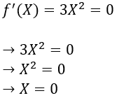Figure — 26: Finding Points Where f’(X)=0

4. Step — 4:

Next, we have only one point where we might have local maxima or minima. Let’s find the second derivative f’’(X) of the function f(X) at the critical point.

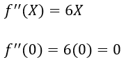Figure — 27: Finding the Second derivative

5. Step — 5:

Since the second derivative at the critical point is 0, we know that at X=0, the test is inconclusive for the concavity of the function. So, now let’s find whether X=0 is an inflection point or not. To do that, we need to test the concavity of f(X) before and after the critical point by selecting a value from an appropriate interval. Here we know that the critical point is 0. So, we need to choose a value from (-∞,0) and (0, ∞). Let’s choose X=-1 and X=1 and see how it goes.

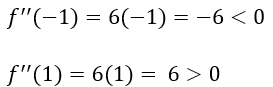Figure — 28: Finding an inflection point

Here, we can see that f’’(X) changes the sign around the point 0. So, we can say that 0 is an inflection point. Other than that, based on the results, we can say that the function is concave in the interval (-∞,0) and convex in the interval (0, ∞).

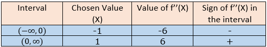Figure — 29: Monitoring the changes in the function

Why Do We Need the First Derivative Test?

Cases When the Second Derivative Test Does Not Work:

• When f’(X) = 0 and f’’(X) = 0.
• When f’(X) = 0 and f’’(X) is not defined.
• When f’(X) is not defined.

In the above cases, we need to use the first derivative test to find out whether the critical point is at a local minimum or at a local maximum.

An example is when the Second Derivative(f’’(X)) is 0 and X is not an Inflection Point:

1. Step — 1:

Our function f(X) is given by…

Figure — 30: Function f(x)

2. Step — 2:

To find the relative extrema(s), we need to find the critical points. Critical points are the points where the first derivative of the function f’(X) = 0.

Figure — 31: Finding the Critical Points of the Function f’(X)

3. Step — 3:

Finding the points where the first derivative of the function (f’(X)) is 0.

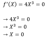Figure — 32: Finding Points Where f’(X)=0

4. Step — 4:

Next, we have only one point where we might have local maxima or minima. Let’s find the second derivative f’’(X) of the function f(X) at the critical point.

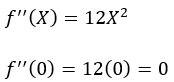Figure — 33: Finding the Second derivative

5. Step — 5:

Since the second derivative at the critical point is 0, we know that at X=0, the test is inconclusive for the concavity of the function. So, now let’s find whether X=0 is an inflection point or not. To do that, we need to test the concavity of f(X) before and after the critical point by selecting a value from an appropriate interval. Here we know that the critical point is 0. So, we need to choose a value from (-∞,0) and (0,∞). Let’s choose X=-1 and X=1, and see how it goes.

Figure — 34: Finding an inflection point

Here we can see that f’’(X) does not change the sign around the point 0. So, we can confidently say that 0 is not an inflection point.

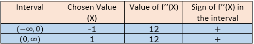Figure — 35: Monitoring the graph on various intervals

Now what?

Now we know that 0 is not an inflection point for f(X) = X⁴. If it is not an inflection point, then it must be either local minima or local maxima. Since the 2nd derivative test failed to determine this, we will apply the 1st derivative test here.

6. Step — 6:

Next, we will choose a point from each of the intervals ((-∞,0) and (0,∞)) and find the value of f’(X) for that chosen point. Here we will also note the sign of f’(X) for the chosen value of X in each interval. If the sign of f’(X) is positive (+), then it means that the function is increasing in that interval. On the other hand, if the sign of f’(X) is negative (-), then it means that the function is decreasing in that interval.

The following table shows the required calculations.

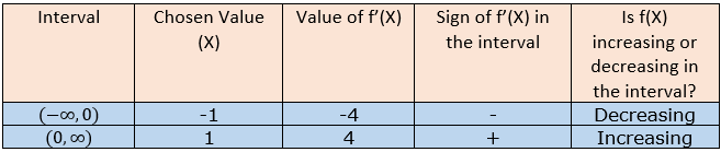Figure — 36: Monitoring the graph on various intervals

From the above table, we can say that the function f(x) is changing from negative to positive. That means that the point X=0 is the local minima for the function f(X)=X⁴.

The First Derivative Test:

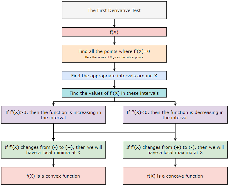Figure 37: The First Derivative Test

The Second Derivative Test:

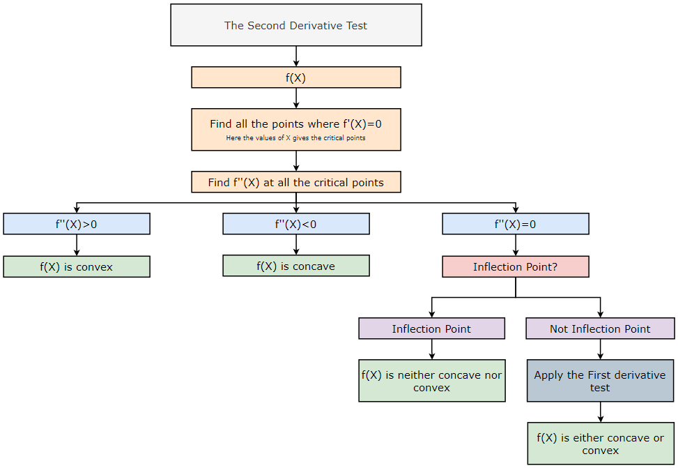Figure — 38: The Second Derivative Test

An Inflection Point Test:

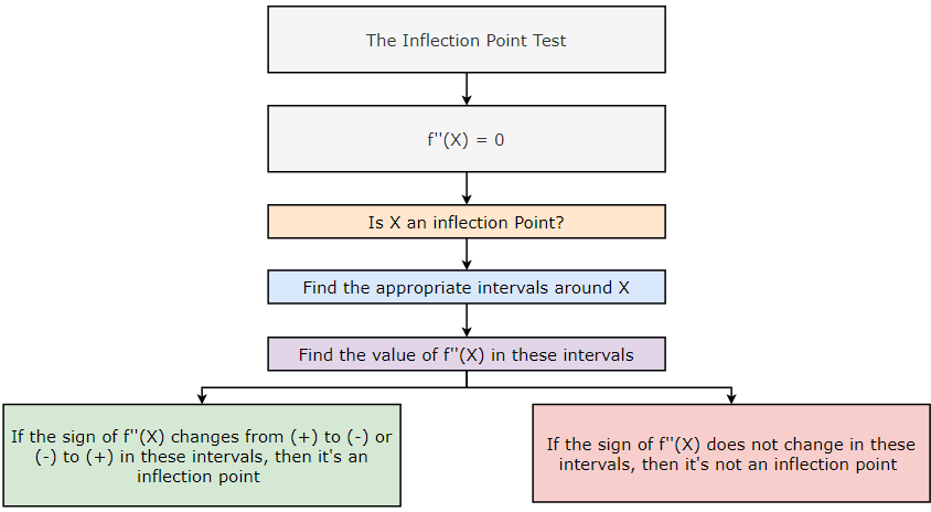Figure-39: An Inflection Point Test

Conclusion:

In conclusion, understanding derivatives is a crucial component of any machine learning practitioner’s toolkit. The ability to analyze and optimize functions using the first derivative test, the second derivative test, and the inflection test can greatly improve the performance of machine learning models. While these concepts may seem daunting at first, with practice and patience, they can become intuitive and even enjoyable to work with. With the rise of deep learning and other complex machine learning techniques, the importance of derivatives is only increasing. By mastering these concepts, you’ll be better equipped to tackle challenging problems in the field and to push the boundaries of what is possible with machine learning.

Citation:

For attribution in academic contexts, please cite this work as:

Shukla, et al., “Mastering Derivatives for Machine Learning”, Towards AI, 2023

BibTex Citation:

@article{pratik_2023, 
 title={Mastering Derivatives for Machine Learning}, 
 url={https://pub.towardsai.net/mastering-derivatives-for-machine-learning-b09336bb074}, 
 journal={Towards AI}, 
 publisher={Towards AI Co.}, 
 author={Pratik, Shukla},
 editor={Binal, Dave}, 
 year={2023}, 
 month={Feb}
}

Resources and References:

1. Derivative — Wikipedia

---

Mastering Derivatives for Machine Learning was originally published in Towards AI on Medium, where people are continuing the conversation by highlighting and responding to this story.

Join thousands of data leaders on the AI newsletter. Join over 80,000 subscribers and keep up to date with the latest developments in AI. From research to projects and ideas. If you are building an AI startup, an AI-related product, or a service, we invite you to consider becoming a sponsor.

Published via Towards AI