Language Modeling From Scratch — Part 2

Author(s): Abhishek Chaudhary

Originally published on Towards AI.

In the previous article we made use of probability distribution to create a name generator, we also looked into using a simple neural network. We concluded the article with the observation that even though a simple neural network with a single character input and single layer didn’t work better than the probabilistic approach, it offers significant flexibility in terms of input dimensionality.

The probability distribution approach increases exponentially in complexity wrt to the input dimension, which is popularly referred to “curse-of-dimensionality”. In this article, we’ll see how neural networks offer us a respite from this situation when we increase the input dimensions.

I highly encourage the readers to go through the previous article before moving further Bigram Language Modeling From Scratch

Code for the article can be found the following jupyter notebook

Training Data

First, we’ll create our training data. Instead of using a single character as input, we’ll make use of triplets to predict the next word. This approach will help the model learn more information from the input and in-turn make better predictions.

words = open('names.txt', 'r').read().splitlines()
character_list = sorted(list(set(''.join(words))))
stoi = {s:i+1 for i,s in enumerate(character_list)} # Adding 1 to each index so that special character can be given index 0
stoi['.'] = 0
itos = {i:s for s,i in stoi.items()} # Create reverse mapping as well
len(words), words[:10]

(32033,
 ['emma',
 'olivia',
 'ava',
 'isabella',
 'sophia',
 'charlotte',
 'mia',
 'amelia',
 'harper',
 'evelyn'])

import torch
import torch.nn.functional as F
import matplotlib.pyplot as plt # for making figures
%matplotlib inline

In the snippet below, we can see how the input triplets and their next character are arranged as training data(X and Y)

# Create training dataset in the form of Xs and Ys
number_of_previous_chars = 3
Xs, Ys = [], []
for word in words[:5]:
 out = [0] * number_of_previous_chars
 for ch in word + '.':
 idx = stoi[ch]
 xStr = "".join([itos[item] for item in out])
 print(f"X: {xStr} Y: {ch}")
 Xs.append(out)
 Ys.append(idx)
 out = out[1:] + [idx]

Xs = torch.tensor(Xs)
Ys = torch.tensor(Ys)
Xs.shape, Ys.shape

X: ... Y: e
X: ..e Y: m
X: .em Y: m
X: emm Y: a
X: mma Y: .
X: ... Y: o
X: ..o Y: l
X: .ol Y: i
X: oli Y: v
X: liv Y: i
X: ivi Y: a
X: via Y: .
X: ... Y: a
X: ..a Y: v
X: .av Y: a
X: ava Y: .
X: ... Y: i
X: ..i Y: s
X: .is Y: a
X: isa Y: b
X: sab Y: e
X: abe Y: l
X: bel Y: l
X: ell Y: a
X: lla Y: .
X: ... Y: s
X: ..s Y: o
X: .so Y: p
X: sop Y: h
X: oph Y: i
X: phi Y: a
X: hia Y: .





(torch.Size([32, 3]), torch.Size([32]))

As we did in the previous article, we can’t use a character index for training. So we’ll convert each character into its one_hot_encoding vector. Since we have 27 characters (26 + ‘.’), each character would be represented by a vector (1,27)

xEnc = F.one_hot(Xs, num_classes=27).float()
xEnc.shape

torch.Size([32, 3, 27])

After we have a character represented as (1,27) tensor, we’d like to embed the character into a lower dimensionality space, for this article we can make use of a 2D space as that would be easy to plot and visualize. We’ll create an Embedding matrix that would then be used to generate Embedded input

Embedding = torch.randn((27, 2))
Embedding.shape

torch.Size([27, 2])

xEmb = xEnc @ Embedding
xEmb.shape

torch.Size([32, 3, 2])

Each character is now represented by (1,2) dimensional tensor

xEmb[0]

tensor([[-1.1452, 1.1325],
 [-1.1452, 1.1325],
 [-1.1452, 1.1325]])

Neural Network

We’ll implement a neural network similar to what’s shown in the image above. We’ll have two hidden layer, one input layer and one output layer. The xEmb would be the output of the input layer and input of hidden layer 1. As we know, each layer in a neural network has associated Weights and Biases; we need W1, W2, and b1, b2 for each layer. The model architecture is taken from Bengio et al. 2003 MLP language model paper

Hidden Layer 1

Input for hidden layer 1 is xEmb of shape (, 3, 2); thus, the input to hidden layer 1 would be of dimension (, 6) as each training sample has 3 characters, and each of the characters is of shape (1,2) embedding. So we’ll define the hidden layer weights as follows

W1 = torch.randn((6, 100))
b1 = torch.randn((100))

If we try to take dot product of W1 and xEmb right now, we’ll get the following error

xEmb @ W1 + b1

---------------------------------------------------------------------------

RuntimeError Traceback (most recent call last)

Cell In[76], line 1
----> 1 xEmb @ W1 + b1


RuntimeError: mat1 and mat2 shapes cannot be multiplied (96x2 and 6x100)

This is because shape of xEmb(32, 3, 2) is not compatible with W1 (6, 100) for dot product. Now we’ll make use of pytorch concept called view, by specifying on dimension as the desired value and -1 for the remaining, pytorch automatically figures out the dimension mentioned as -1

xEmb.shape, xEmb.view(-1, 6).shape

(torch.Size([32, 3, 2]), torch.Size([32, 6]))

Now the matrices are compatible for dot product and we can make use of the neural network equation to get the output of hidden layer 1

h1 = xEmb.view(-1, 6) @ W1 + b1
h1.shape

torch.Size([32, 100])

Hidden Layer 2

Similar to hidden layer 1, we’ll initialize W2 and b2. Input to HL2 would be the output of HL1, i.e., h1. The output of the last hidden layer is termed as logits (log-counts as we discussed in the previous article)

W2 = torch.randn((100, 27))
b2 = torch.randn((27))

logits = h1 @ W2 + b2
logits.shape

torch.Size([32, 27])

To convert log counts or logits to actual counts, we’ll perform exp operation and then normalize along column the counts to get the probability of each character in the output.

count = logits.exp()
probs = count / count.sum(1, keepdim=True)
probs.shape

torch.Size([32, 27])

To verify that the above operation was correct, we can check that the sum along the column for a row should be 0

probs[0].sum()

tensor(1.)

Cross Entropy Loss

In the previous article, after getting the probabilities, we were getting the probability of the expected character from the output. To obtain a continuous smooth distribution, we then took a log of the probability and calculated the sum of that log. In ideal situation, the probability of expected character should be 1, resultant log should be 0 and sum of logs of probabilities should 0 as well. So, we use the sum of the log of probabilities as our loss function. Since a lower probability would result in the lower log, we take the negative of the log and term it as a negative log-likelihood. This is also called cross-entropy loss.

import numpy as np
x = np.linspace(0.000001, 1, 100)
y = np.log(x)
plt.plot(x, y, label='y = log(x)')

[<matplotlib.lines.Line2D at 0x12ec14150>]

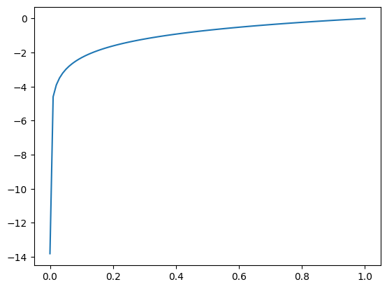
One disadvantage of implementing this method as is, is that for very low probability log approaches -inf, resulting in loss to be infinity. This is considered weird and generally disliked in the community, so instead, we use pytorch implementation of cross_entropy. Pytorch adds a constant to each probability which prevents it from getting very low, hence smoothening out the log and trapping the log function, keeping it from going to inf

loss = F.cross_entropy(logits, Ys)
loss

tensor(51.4781)

Using the entire dataset

# Training dataset
number_of_previous_chars = 3
Xs, Ys = [], []
for word in words:
 out = [0] * number_of_previous_chars
 for ch in word + '.':
 idx = stoi[ch]
 xStr = "".join([itos[item] for item in out])
 Xs.append(out)
 Ys.append(idx)
 out = out[1:] + [idx]

Xs = torch.tensor(Xs)
Ys = torch.tensor(Ys)
Xs.shape, Ys.shape

(torch.Size([228146, 3]), torch.Size([228146]))

g = torch.Generator().manual_seed(2147483647) # for reproducibility
xEnc = F.one_hot(Xs, num_classes=len(character_list)+1).float()

embedding = torch.randn((len(character_list)+1, 10), generator=g)
W1 = torch.randn((30, 200), generator=g) # (3*2, 100)
b1 = torch.randn(200, generator=g) 
W2 = torch.randn((200, 27), generator=g)
b2 = torch.randn(27, generator=g)

parameters = [embedding, W1, b1, W2, b2]

Setting each of parameters as ‘requires_grad’ so that pytorch uses those in back-propagation

for p in parameters:
 p.requires_grad = True
sum(p.nelement() for p in parameters)

11897

Training

Setting a training loop for 200000 steps, with a learning rate of 0.1, which decided how big of an update to be done to the parameters. We also track the loss and steps to later plot how loss varies with steps. We also make use of mini-batches of size 32 to speed up the training process.

lr = 0.1
lri = []
lossi = []
stepi = []
for i in range(400000):
 # Define one hot encoding, embedding and hidden layer
 miniBatchIds = torch.randint(0, Xs.shape[0], (32,)) # Using a minibatch of size 32
 xEmb = xEnc[miniBatchIds] @ embedding
 h = torch.tanh(xEmb.view(-1, 30) @ W1 + b1)
 logits = h @ W2 + b2
 loss = F.cross_entropy(logits, Ys[miniBatchIds])

 # backward pass
 for p in parameters:
 p.grad = None
 loss.backward()

 lr = 0.1 if i < 100000 else 0.01
 for p in parameters:
 p.data += -lr * p.grad

 stepi.append(i)
 lossi.append(loss.log10().item())

print(loss.item())

2.167637825012207

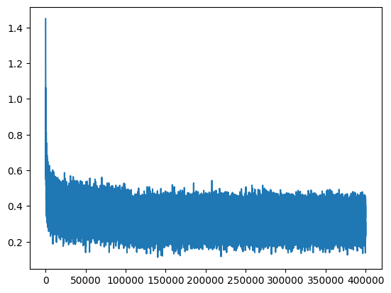
The learning plot below has a thickness associated with it, that’s because we are optimizing on mini-batches

plt.plot(stepi, lossi)

[<matplotlib.lines.Line2D at 0x12e253090>]

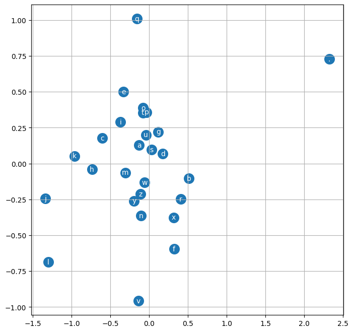
We can also visualize the embedding we have created while training.

# visualize dimensions 0 and 1 of the embedding matrix C for all characters
plt.figure(figsize=(8,8))
plt.scatter(embedding[:,0].data, embedding[:,1].data, s=200)
for i in range(embedding.shape[0]):
 plt.text(embedding[i,0].item(), embedding[i,1].item(), itos[i], ha="center", va="center", color='white')
plt.grid('minor')

Inference

Let’s try to generate 10 names using our model and compare them with the names generated using previous models

# sample from the model
g = torch.Generator().manual_seed(2147483647 + 10)

for _ in range(10):
 out = []
 context = [0] * number_of_previous_chars # initialize with all ...
 while True:
 emb = embedding[torch.tensor([context])] # (1,block_size,d)
 h = torch.tanh(emb.view(1, -1) @ W1 + b1)
 logits = h @ W2 + b2
 probs = F.softmax(logits, dim=1)
 ix = torch.multinomial(probs, num_samples=1, generator=g).item()
 context = context[1:] + [ix]
 out.append(ix)
 if ix == 0:
 break
 
 print(''.join(itos[i] for i in out))

mora.
mayah.
seen.
nihahalerethrushadra.
gradelynnelin.
shi.
jen.
eden.
van.
narahayziqhetalin.

Conclusion

Names generated by the above models are more “name-like” than the previous model, as we have better information about the patterns. This can be attributed to

• Better input provided to the model: The neural network is able to model the relationship between multiple input characters and then predict the next character. As opposed to the probability distribution, neural network handles the “curse-of-dimensionality” better
• More complex model: Our current neural network is more complex than the one we discussed earlier and is able to learn better.

With our previous approach, we achieved a loss of 2.5107581615448, while with our current model, we went down to 2.167637825012207.

Join thousands of data leaders on the AI newsletter. Join over 80,000 subscribers and keep up to date with the latest developments in AI. From research to projects and ideas. If you are building an AI startup, an AI-related product, or a service, we invite you to consider becoming a sponsor.

Published via Towards AI