Introduction to Reinforcement Learning Series. Tutorial 3:…

For example, if we’re designing an agent to control an autonomous car, we can’t perfectly predict the future state. This is because we don’t have a perfect model of how other cars and pedestrians will move or react to our movements.

How the state evolves in response to our actions is defined by the state transition function. This can be stochastic (based on probabilities) or deterministic (not based on probability). In the autonomous driving example, this is simply how the state will evolve over time — how other road users will move. For this example, it’s hard to imagine what this function would look like. The state transition function for chess is much simpler — the board changes from how it was before your move to how it looks after your move.

When we don’t know the state transition function, we can’t plan ahead perfectly and work out what the optimal action is in each situation, because we don’t know what the outcomes of our actions will be.

However, what we can do is interact with the environment and learn from our experience in it. By taking action in the environment, and seeing their results (how the state changes and any rewards we get), we can improve our future action selection.

Training & Testing in RL (compared with Machine Learning)

Typically in machine learning, you train your machine learning model on a fixed training dataset and then test it on another completely distinct fixed dataset. The testing step evaluates how well the ML model generalizes to data your model hasn’t been able to train on.

These paradigms still exist in RL but are much more blurred. To train with reinforcement learning, you need to interact with the real environment. And while you do so, you’re also able to see how well it achieves the task you’ve set for it. So while training RL, you’re both evaluating it and improving its ability simultaneously.

Aside: this isn’t the case in a multi-agent scenario if the agents you train with aren’t the same as the agents you will play against in ‘testing’. Keep this in mind for the competitions!

2. Temporal-Difference Learning

Temporal-Difference (TD) Learning is the first Reinforcement Learning algorithm we’re introducing.

It learns a value function estimate directly from interacting with the environment — without needing to know the state transition function.

In Tutorial 2, we saw that the value function changes based on which policy we follow. Stated more concretely, following one policy will give us a different value (expected return) from each state than another.

TD Learning estimates the value function for a given policy, π.

TD Learning is an ‘online’ learning algorithm. This means it learns after every step of the experience. This is in contrast to algorithms that interact with the environment for some time to gather experience, and then learn based on that.

Here’s the basic logic of the TD Learning algorithm:

Initialize the value function estimate with arbitrary values (for example, set to 0) for all states
Initialize the environment
Get the action using our estimate of the value of state s
Observe the reward and next state from the environment (decided by the reward function and state transition function respectively)
Update the value function estimate for that state using the TD Update Equation (see below)
Go back to step 3. until the episode ends

2.1 Temporal Difference Update Equation

The update equation is based on the Bellman Equation, so we’re restating this first:

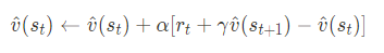
While not the typical way that the TD Update Equation is shown, below is the way we think is most intuitively understandable. There’s a lot of notation here that may be new to you, which is hopefully well-explained in the toggles below

Note: the arrow in ????^(????????)←expressionv^(st)←expression simply means the expression on the right is updating our estimator on the left side of the arrow — the value function estimate for this state.

Let’s briefly consider each term in this expression:

▼v^(st)

It is our value function estimate for our current policy for state st.
The little hat over the v simply means it’s an estimate, rather than the true value function of the current policy.

▼ The step-size parameter α

It is a number where 0<α<1.
A typical example that can be used in the exercises we’ll face is 0.2.
This affects how quickly the value function converges to the optimal value. Larger α converges faster but too large, and learning can be unstable!

Interpretation: this has 2 main terms:

(1−α)v^(st) — mostly use the previous estimate, but we remove a small proportion of it (α, which is between 0 and 1)
α[rt+γv^(st+1)] — replace the small part we removed with the value ‘experienced’ — ie replace αv^(st) with this (this just plugs in the Bellman Equation!)

U+27A4 The typical way the TD Update Equation is shown is a little different

U+27A4 We can express the right-hand side as ????(????????) + αδt

▼ δt is the TD-error, where δt = rt + γv ^ (st+1) − v^(st)

It’s the difference between our original estimate of the value of state st and our new estimate based on the reward we’ve observed rt and the value estimate of the next state we’ve reached v^(st+1).

The above rewriting of the right-hand side is common in machine learning when updating an ML model based on a ‘loss’ (1) and using a step-size hyperparameter (α ).

(1) Loss functions are used in other flavors of machine learning to measure how well a machine learning model makes predictions. Also, knowing its performance allows you to improve it.

2.2 TD-Learning algorithm in pseudocode

You’ll want to check this when you’re completing the exercises! Read through it and try to understand it first, though.

FOR episode_number in number of episodes you'd like to run:

 Sample starting state

 WHILE episode hasn't terminated

 Sample action from policy(state)

 Sample next_state from transition_function(state, action)

 Sample reward from reward_function(state, action, next_state)

 UPDATE value_function using TD update rule

 UPDATE state to next_state

 END WHILE

END FOR

Since TD Learning is an online algorithm, it learns during episodes, after each step of the experience. It updates its estimates of values in an ongoing process based on estimates of other states (the v^(st+1) term). This is known as 'bootstrapping'.

Review:

1. In what sense does TD Learning do “bootstrapping”?

U+27A5 It learns by updating estimates of value (v^(st)) using estimates of other states’ values (v^(st+1)).

2. What does the hat over the v in v^(st) denote for a value function?

U+27A5That it is an estimate, not the true value.

3. How should we interpret the two terms of the TD Update Equation,v^(st) ← (1−α) v^ (st) + α[rt + 1 + γv^(st+1)]?

U+27A5 We take the weighted sum of

(1) the previous estimate and

(2) the value we just experienced.

4. What three things happen in each step of the TD Learning algorithm?

U+27A5 Choose an action using our policy; observe the reward and successor state from the environment; update the value function estimate using the TD Update Equation.

5. What does TD Learning estimate?

U+27A5 The value function for a given policy.

6. What does TD Learning an abbreviation for?

U+27A5Temporal-Difference Learning

7. What’s a typical value for α in TD Learning?

U+27A50.2.

8. In what sense does RL blur the training and testing phases of traditional ML?

U+27A5While training an RL agent, you’re evaluating it and improving its ability simultaneously.

9. What does it mean that TD Learning is an “online” learning algorithm?

U+27A5It learns after every step, not by retrospectively analyzing bulk data.

10. Why might it be hard to determine an RL environment’s state transition function?

U+27A5e.g. for a self-driving car, you lack a perfect model of how other cars will move

11. What does α represent in the TD Update Equation?

U+27A5The step size parameter is a number where 0<α<1. Large values give more weight to the most recent estimates.

12. Give the TD Update Equation.

U+27A5v^(st) ← (1−α) v^(st) + α[rt+1 + γv^(st+1)]

13. How can you estimate a policy’s value function without knowing the state transition function?

U+27A5e.g. by taking actions in an environment and directly observing the resulting state

3. The `Env` class

Below is the code for the Env class, which has the same interfaces (same function names & return types) as OpenAI Gym's Env class. OpenAI Gym has many classic games and puzzles for RL algorithms already implemented in code, so we use these from time to time in the exercises.

U+27A4 New to Python classes?

We haven’t built a tutorial or exercises for this, but we recommend this short explainer of Python classes.
Just so it’s clear what you do and don’t need to know, make sure you understand everything in this free online interactive tutorial

Since this Env class is very commonly used in RL in Python, we're using it throughout the course. Please read through the below parent class's docstrings carefully and understand the 3 functions that are implemented in all Env subclasses.

The concrete example Env class that follows (FlightPathEnv) may help you understand this better.

from typing import Dict, Tuple, Any
class Env:
 def __init__(self):
 """
 Initialises the object.

 Is called when you call `environment = Env()`.

 It sets everything up in the starting state for the episode to run.
 """
 self.reset()


def step(self, action: Any) -> Tuple[Any, float, bool, Dict]:
 """
 Given an action to take:
 1. sample the next state and update the state
 2. get the reward from this timestep
 3. determine whether the episode has terminated


 Args:
 action: The action to take. Determined by user code
 that runs the policy


 Returns:
 Tuple of:
 1. state (Any): The updated state after taking the action
 2. reward (float): Reward at this timestep
 3. done (boolean): Whether the episode is over
 4. info (dict): Dictionary of extra information
 """
 raise NotImplementedError()

def reset(self) -> Tuple[Any, float, bool, Dict]:
 """
 Resets the environment (resetting state, total return & whether
 the episode has terminated) so it can be re-used for another
 episode.


Returns:
 Same type output as .step(). Tuple of:
 1. state (Any): The state after resetting the environment
 2. reward (None): None at this point, since no reward is 
 given initially
 3. done (boolean): Always `False`, since the episode has just
 been reset
 4. info (dict): Dictionary of any extra information
 """
 raise NotImplementedError()

How can I use this in Python?

environment = Env() # Got to initialise the Env

# Running 100 episodes...
 for episode_num in range(100):
 # You have to .reset() the Env every episode!
 state, reward, done, info = environment.reset()

# Keep going until it terminates - if there's no terminal state then
# it'll keep going forever, so you would insert a 'break' in the loop!
 while not done:
 action = ... # Pick an action based on a policy

 # Step forward in time, simulating the MDP
 state, reward, done, info = environment.step(action)

This code is provided for you in the below exercise U+1F603

3.1 Concrete example: `FlightPathEnv`

class FlightPathEnv(Env):
 """
 You need to use this FlightPathEnv class to learn the 
 optimal value function.
 """
 
 # This defines the possible cities to fly to from each city
 POSS_STATE_ACTION = {
 "New York": ["London", "Amsterdam"],
 "London": ["Cairo", "Tel Aviv"],
 "Amsterdam": ["Tel Aviv", "Cairo"],
 "Tel Aviv": ["Bangkok", "Cairo", "Hong Kong"],
 "Cairo": ["Bangkok"],
 "Bangkok": ["Hong Kong"],
 "Hong Kong": []
 }


# The values define the time to fly from the 1st city in the 
# tuple to the 2nd. E.g. New York -> Amsterdam takes 7.5 hours
 REWARDS = {
 ("New York", "Amsterdam"): -7.5,
 ("New York", "London"): -6,
 ("London", "Cairo"): -8,
 ("London", "Tel Aviv"): -8,
 ("Amsterdam", "Cairo"): -10,
 ("Amsterdam", "Tel Aviv"): -4,
 ("Tel Aviv", "Cairo"): -2,
 ("Tel Aviv", "Bangkok"): -8,
 ("Tel Aviv", "Hong Kong"): -13,
 ("Cairo", "Bangkok"): -4.5,
 ("Bangkok", "Hong Kong"): -1.5,
 }

def __init__(self):
 """Initialise the environment"""
 self.reset()

def reset(self) -> Tuple[str, float, bool, Dict]:
 """
 Reset the environment, allowing you to use the same FlightPathMDP object
 for multiple runs of training.
 """
 self.state = "New York"
 self.total_return = 0
 self.done = False
 return self.state, self.total_return, self.done, {}

def check_new_state_is_valid(self, new_state: str) -> None:
 """
 Check that a state transition is valid based on
 which cities can be flown to from where.
 """
 assert new_state in self.POSS_STATE_ACTION, \
 f"{new_state} is not a valid state to fly to"
 assert new_state in self.POSS_STATE_ACTION[self.state], \
 f"You can't fly from {self.state} to {new_state}. Options: {self.POSS_STATE_ACTION[self.state]}"

def step(self, action: str) -> Tuple[str, float, bool, Dict]:
 """
 Given an action to take, update the environment and give the reward.
 """
 # In this case the actions and new states are the same.
 # THIS IS NOT ALWAYS THE CASE.
 new_state = action

 self.check_new_state_is_valid(new_state)
 
 # Get the reward at this timestep (the time taken to make this flight)
 reward = self.REWARDS[(self.state, new_state)]

 # Add the reward from flight to the total
 self.total_return += reward

 # Update the state to the new state
 self.state = new_state
 
 # The game is over if you've reached Hong Kong
 self.done = self.state == "Hong Kong"

 return self.state, reward, self.done, {}

4. Exercise: Learning a Value Function from Experience!

https://replit.com/team/delta-academy-RL7/31-Learning-a-value-function-from-experience

Let’s get concrete & find the value function from experience in an environment!

We’re again going to calculate the optimal value function for the flight path MDP we’ve seen before, but this time we’ll learn it from interacting with an Env environment.

Once you’ve finished…

You should notice that the value of London is 0. Why is this?

U+27A4Answer

It’s 0 because this state hasn't been visited during training since it's not on the path from New York to Hong Kong taken by the optimal value function.

This presents a problem if you’re trying to learn the optimal value function through experience for all states and always take the same paths during training. For example, if you learn the current policy’s value function with TD and then act ‘greedily’ (pick the action with the highest successor state value ).

You need your algorithm to sometimes explore new states…

5. Exploration-Exploitation Trade-off

A critical trade-off to understand when designing reinforcement learning algorithms is the trade-off between exploration and exploitation.

The most effective way for an agent to gain reward is to take actions that in the past have yielded rewards. This exploits its existing knowledge of the environment.

However, unless the agent already knows the optimal policy, there may be unexplored actions that lead to greater rewards. To discover better actions, the agent must try actions with unknown outcomes. This is exploring.

Successful actions discovered through exploration can then be exploited when the option of moving to that state is encountered again.

Should the robot exploit the usual place he likes? Or explore? (Source: UC Berkeley CS188)

This dichotomy exists in real life too — do you try a new restaurant, or go to your old favorite? Perhaps the new one will become your new favorite — you’ll never know if you don’t try!

Doing all of one or the other isn’t great — you won’t enjoy trying every single restaurant in the city, but if you always go to your childhood favorite, you’ll never find new things you like. The same is true in RL. An agent which only exploits or only explores tends to perform badly. Hence some amount of both of these two behaviors must be incorporated into the algorithm during training.

This is the exploration-exploitation trade-off.

5.1 Action-Values

Suppose we want to decide which action a to take from the current state s. We introduce the concept of the action-value function to do this. The action value is a number associated with a state-action pair (s, a). The action-value function is usually denoted qπ(s, a).

The action-value qπ(s,a) for state-action pair (s,a) is the value associated with taking action a from state s and then following policy π .

For now, we’ll calculate action values using a “1-step lookahead”. Instead of calculating the value function by looking many steps into the future, we can just look 1 step into the future and use the value function estimate v^(s).

First, what is meant by “looking 1 step into the future”? In short, we use the reward function and the transition function. The reward function lets us see the reward we would receive after taking action a . Similarly, the transition function lets us see the successor state we would transition to after taking action a.

A 1-step lookahead simply uses Bellman’s Equation as follows:

Notation

q^(s, a) is the action-value function
′s′ is the successor state — the state we transition to after being in state s and taking action a
r(s,a,s′) is the reward when transitioning from state s to state ′s′ after taking action a
γ is the time discount factor
v^(s′) is the value function for the successor state

5.2 Greedy Actions

The greedy action is the action that has the highest action value for that state, according to your current value function estimate.

U+27A4 Stated mathematically

Taking greedy actions is exploitation as you exploit your existing knowledge of the environment to gain a reward.

Taking a non-greedy action is exploration, as, though it may not lead to immediate reward, it may improve the policy and maximize future rewards.

5.3 ϵ -greedy

One common way to address this tradeoff when designing our algorithm is to be greedy most of the time, but take a random non-greedy action some of the time, with a fixed probability. This approach to exploration is termed ϵ -greedy (Greek lowercase letter epsilon), where epsilon ϵ is the probability of taking a random action (exploring).

Stated mathematically, this is:

This is only used during training. If you want your agent to perform its best, you make it act purely greedily.

A good value of ϵ is different for different tasks. In small environments with few states, a relatively high value of ϵ will work well as exploration will quickly lead to the discovery of high-reward actions. However, in a large environment with ‘sparse’ (1) rewards, a greedier approach with a lower ϵ may be better as exploration will waste a lot of turns exploring low-reward states.

(1) ‘Sparse’ rewards mean rewards are rare. Most states are undifferentiated (give 00 rewards, for example), while a very limited number do give rewards.

6. Exercise: Keep Barry Happy!

https://replit.com/team/delta-academy-RL7/32-Keep-Barry-happy

Business is booming for BarryJet! To celebrate, Barry decides to take 10,000 flights on his planes. He has a fleet of 100 planes and wants to have the best experience possible across all 10,000 flights.

Barry scores his experience by awarding Barry points at the end of each flight. Each plane is different, so Barry finds them differently rewarding.

However there is some randomness in the flight experience, sometimes a plane’s flight crew is having a good day and sometimes they aren’t! So the same plane may not get the same number of Barry points for all flights.

Your task is to balance the exploration of new planes with the exploitation of the best planes seen so far!

7. Terminal State’s Value

One thing we’ve not discussed is how to set the value estimate for the terminal state in TD-Learning. Terminal states don’t have a successor state, so the TD-Learning Update can’t be used. As a recap, the value is defined as the expected future return from this state.

As a result, the value of any terminal state is 00 since no rewards follow it.

Let’s suppose we’re in an environment where you receive a reward for 0 every timestep except when you move into the terminal state when you receive a +1 reward. This is visualized below.

Example MDP showing how the terminal state should be set. Actions & state transitions are shown as red arrows, while rewards are green text next to the arrows. The values are above each state, color-coded.

If the discount factor, γ is 0.99, the value of being in the state preceding the terminal state would be 11 when following the optimal policy. This is because the return from being in this state, when following the optimal policy, is the reward we receive when moving to the terminal state.

What about the action values we use for action selection? Won’t it be an issue if the terminal state’s value is 00? Let’s look at the two action values for the penultimate state in the above example.

There are 2 possible actions:

Move to a 3rd-last state
Move to the Terminal state

The action value for moving to the 3rd-last state, given we’re in the penultimate state, is:

0 + 0.99 × 0.99 = 0.981

Whereas, the action value for moving to the Terminal state, given we’re in the penultimate state, is:

1 + 0.99 × 0 = 1

As a result, greedy action selection using 1-step lookahead selects moving to the terminal state, which is intuitively the right action to take.

Review:

1. How does an ϵ -greedy strategy apply differently in training vs. in performance?

U+27A5 In performance, the agent should act purely greedily.

2. When might lower vs. higher values of ϵ in ϵ-greedy algorithms make sense?

U+27A5 Higher values are better when there are relatively few states since that will assure the agent will quickly visit them all; lower values are better when there are many states, but only very few with a good reward.

3. What’s meant by “exploitation” in RL, in the context of the explore-exploit trade-off?

U+27A5 Taking the action which historically yielded the highest return (i.e. the greedy action).

4. Give a definition in words of the action-value function, qπ(s, a).

U+27A5 The value associated with taking action a from state s and then the following policy π.

5. What is the value of a terminal state in a Markov decision process?

U+27A5 0.

6. Why is it necessary to balance exploration and exploitation when training RL agents?

U+27A5 An agent which only exploits its best-guess policy may never explore a chain of actions that would produce a better return; an agent which only explores may spend much of its time in suboptimal states.

7. Give the equation of an action-value function that uses a 1-step lookahead.

U+27A5 q^(s,a) = r(s,a,s′) + γ × v^(s′)

8. What does qπ denote in a Markov decision process?

U+27A5 The action-value function.

9. What is an ϵ-greedy strategy in RL?

U+27A5 Explore (e.g. randomly) with probability ϵ; exploit (i.e. take the greedy action) with probability 1−ϵ.

10. What’s the greedy action in RL?

U+27A5 The action with the highest estimated action value for that state.

11. What’s meant by “exploration” in RL, in the context of the explore-exploit trade-off?

U+27A5 Trying under-explored actions which might yield greater returns.

8. Exercise: Barry’s Parking Predicament!

https://replit.com/team/delta-academy-RL7/33-Barrys-Parking-Predicament

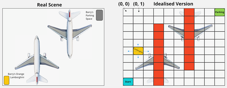
Barry drives an orange Lamborghini. Since he’s such a baller he parks in the airport hangar next to where several of his BarryJet planes are kept. (See left side of diagram)

He’s in the bottom left corner of the hangar (viewed from above). He wants to park his car in the top right corner but needs to navigate around the two parked planes to do so.

The right side of the diagram shows an idealized version of the problem, which we’re going to solve by writing our first Reinforcement Learning algorithm.

The hangar has been divided into grid squares. Barry wants to drive from the bottom left square to the top right. He cannot drive underneath the planes (although can go under the wings). The grid squares he can’t drive through are shown in red.

You want to iteratively update the value function approximation using TD-learning while using ???? -greedy to ensure the explore-exploit tradeoff is well balanced.

Join thousands of data leaders on the AI newsletter. Join over 80,000 subscribers and keep up to date with the latest developments in AI. From research to projects and ideas. If you are building an AI startup, an AI-related product, or a service, we invite you to consider becoming a sponsor.

Published via Towards AI

Cookie	Duration	Description
cookielawinfo-checkbox-analytics	11 months	This cookie is set by GDPR Cookie Consent plugin. The cookie is used to store the user consent for the cookies in the category "Analytics".
cookielawinfo-checkbox-functional	11 months	The cookie is set by GDPR cookie consent to record the user consent for the cookies in the category "Functional".
cookielawinfo-checkbox-necessary	11 months	This cookie is set by GDPR Cookie Consent plugin. The cookies is used to store the user consent for the cookies in the category "Necessary".
cookielawinfo-checkbox-others	11 months	This cookie is set by GDPR Cookie Consent plugin. The cookie is used to store the user consent for the cookies in the category "Other.
cookielawinfo-checkbox-performance	11 months	This cookie is set by GDPR Cookie Consent plugin. The cookie is used to store the user consent for the cookies in the category "Performance".
viewed_cookie_policy	11 months	The cookie is set by the GDPR Cookie Consent plugin and is used to store whether or not user has consented to the use of cookies. It does not store any personal data.

Frequently Used, Contextual References

Resources

Publication

Introduction to Reinforcement Learning Series. Tutorial 3: Learning from Experience, TD-Learning, ϵ -Greedy

Author(s): Towards AI Editorial Team

Table of Content:

1. Learning from Experience

Training & Testing in RL (compared with Machine Learning)

2. Temporal-Difference Learning

2.1 Temporal Difference Update Equation

2.2 TD-Learning algorithm in pseudocode

3. The Env class

How can I use this in Python?

3.1 Concrete example: FlightPathEnv

4. Exercise: Learning a Value Function from Experience!

Once you’ve finished…

5. Exploration-Exploitation Trade-off

5.1 Action-Values

5.2 Greedy Actions

5.3 ϵ -greedy

6. Exercise: Keep Barry Happy!

7. Terminal State’s Value

Review:

8. Exercise: Barry’s Parking Predicament!

Related posts

Feedback ↓ Cancel reply

Popular posts

Updates

Recent Posts

The World’s Leading AI and Technology Publication.

Company

CONTACT US

GDPR CCPA Statement

3. The `Env` class

3.1 Concrete example: `FlightPathEnv`