Introduction to Neural Networks and Their Key Elements (Part-C) — Activation Functions & Layers

Last Updated on June 19, 2020 by Editorial Team

Author(s): Irfan Danish

Machine Learning

Introduction to Neural Networks and Their Key Elements (Part-C) — Activation Functions & Layers

In the previous story we have learned about some of the hyper parameters of an Artificial Neural Network. Today we’ll talk about activation functions and Layers, which some people may consider them hyper-parameters and some not.

So let’s begin today's story.

1. Activation Function

To understand about activation function first we need to recall the artificial neuron. So what does an artificial neuron do? Simply put, it calculates a “weighted sum” of its input, adds a bias and then decides whether it should be “fired” (activated) or not ( yeah right, an activation function does this, but let’s go with the flow for a moment ).

So consider a neuron.

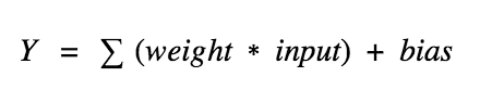
Now, the value of Y can be anything ranging from -inf to +inf. The neuron really doesn’t know the bounds of the value. So how do we decide whether the neuron should fire or not ( why this firing pattern? Because we learned it from biology that’s the way brain works and the brain is a working testimony of an awesome and intelligent system ).

We decided to add “activation functions” for this purpose. To check the Y value produced by a neuron and decide whether outside connections should consider this neuron as “fired” or not. Or rather let’s say — “activated” or not.

These are also known as mapping functions. They take some input on the x-axis and output a value in a restricted range(mostly). They are used to convert large outputs from the units into a smaller value most of the time and promote non-linearity in your NN. Your choice of an activation function can drastically improve or hinder the performance of your NN. You can choose different activation functions for different units if you like.

Now lets take a simple example:

The first thing that comes to our minds is how about a threshold based activation function? If the value of Y is above a certain value, declare it activated. If it’s less than the threshold, then say it’s not. Hmm great. This could work!

Activation function A = “activated” if Y > threshold else not

Alternatively, A = 1 if y> threshold, 0 otherwise

Well, what we just did is a “step function”, see the below figure.

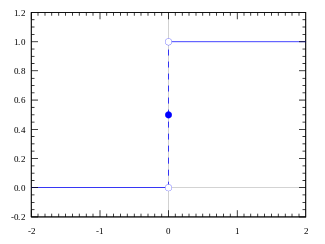
Its output is 1 ( activated) when value > 0 (threshold) and outputs a 0 ( not activated) otherwise. Great. So this makes an activation function for a neuron.

Now lets talk about more realistic or most used activation functions in Deep Learning practices.

1.1. tanh Activation Function:

The tanh activation is used to help regulate the values flowing through the network. The tanh function squishes values to always be between -1 and 1.

The tanh activation is used to help regulate the values flowing through the network. The tanh function squishes values to always be between -1 and 1.

When vectors are flowing through a neural network, it undergoes many transformations due to various math operations. So imagine a value that continues to be multiplied by let’s say 3. You can see how some values can explode and become astronomical, causing other values to seem insignificant.

A tanh function ensures that the values stay between -1 and 1, thus regulating the output of the neural network. You can see how the same values from above remain between the boundaries allowed by the tanh function.

1.2. Sigmoid Activation Function:

A sigmoid activation is similar to the tanh activation. Instead of squishing values between -1 and 1, it squishes values between 0 and 1. That is helpful to update data because any number getting multiplied by 0 is 0, causing values to disappears or be “forgotten.” Any number multiplied by 1 is the same value therefore that value stay’s the same or is “kept.” The network can learn which data is not important therefore can be forgotten or which data is important to keep. The neurons which have values near to zero will have less impact and the neurons which produces values near to 1 will have more impact.

Sigmoid, is mostly used in output neurons in case of binary classification problem to convert the incoming signal into a range of 0 to 1 so that it can be interpreted as a probability.

Do not mix the sigmoid with softmax because in sigmoid all the neurons have values between 0 and 1 and it is possible that the sum of the values of all neurons may not be equal to 1.

1.3. Softmax Activation Function:

Softmax function comes from the family of Sigmoid functions only. Softmax is a wonderful activation function that turns numbers often known as logits into probabilities that sum to one. Softmax function outputs a vector that represents the probability distributions of a list of potential outcomes.

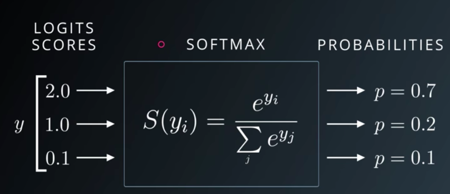
Softmax function squashes the incoming signals for multiple classes in a probability distribution. The sum of this probability distribution would obviously be 1. It is mostly used in multi class classification.

1.4. ReLU Activation Function:

The ReLU is the most used activation function in the world right now. Since it is used in almost all the convolutional neural networks or deep learning. ReLU stands for a rectified linear unit. If you are unsure what activation function to use in your network, ReLU is usually a good first choice.

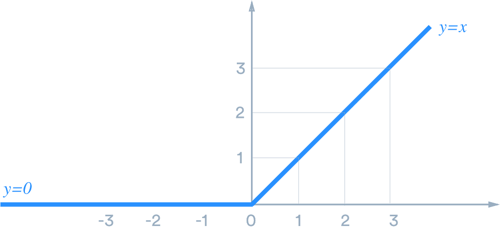
ReLU is linear (identity) for all positive values, and zero for all negative values. What it means is that all the values greater than 0 are not transformed, they just stay as it is. And values less than zero or negative values will be transformed to zero.

It’s cheap to compute as there is no complicated math. The model can therefore take less time to train or run. It converges faster.

Linearity means that the slope doesn’t plateau, or “saturate,” when x gets large. It doesn’t have the vanishing gradient problem suffered by other activation functions like sigmoid or tanh.

The downside for being zero for all negative values is a problem called “dying ReLU.” A ReLU neuron is “dead” if it’s stuck in the negative side and always outputs 0. The dying problem is likely to occur when the learning rate is too high or there is a large negative bias. Lower learning rates often mitigates the problem. If not, Leaky ReLU, Parameteric ReLU, and ELU are also good alternatives to try. They have a slight slope in the negative range, thereby preventing the issue.

2. Layers

Artificial Neural Network is a computing system inspired by a biological neural network that constitute the animal brain. Such systems “learn” to perform tasks by considering examples, generally without being programmed with any task-specific rules.

These are what help a Neural Network gain complexity in any problem. Increasing layers (with units) can increase the non-linearity of the output of a Neural Network.

Each layer contains a number of Units/Neurons. The amount in most cases is entirely up to the creator. However, having too many layers for a simple task can unnecessarily increase its complexity and in most cases decrease its accuracy. The opposite also holds true.

The Neural Network is constructed from 3 type of layers:

1. Input layer — initial data for the neural network.
2. Hidden layers — an intermediate layer between input and output layer and place where all the computation is done.
3. Output layer — produce the result for given inputs.

There are 3 blue circles on the image above. They represent the input layer and usually are noted as vector X. There are 4 yellow and then 3 yellow circles again that represent the hidden layers. These circles represent the “activation” nodes and usually are noted as W or θ. The green circles are the output layer or the predicted value (or values in case of multiple output classes/types).

Each node is connected with each node from the next layer and each connection (black arrow) has a particular weight. Weight can be seen as an impact that that node has on the node from the next layer. So if we take a look on one node it would look like this

Let’s look at the top yellow node (“Fig 1”) in the first hidden layer. All the nodes from the previous layer (blue) are connected with it. All these connections represent the weights (impact). When all the node values from the blue (input) layer are multiplied with their weight and all this is summarised it gives some value for the top yellow node. The yellow node has predefined “activation” function (tanh in “Fig 2”) which defines if this node will be “activated” or how “active” it will be, based on the summarised value. The additional node with value 1 is called the “bias” node.

A Neural Network with 2 or more hidden layers with each layer containing many units/neurons is called a Deep Neural Network which is why this field is named Deep Learning.

So that was it for this story in the next story we will learn about the learning process of Neural Networks.

To see my work you can follow me on Github & Medium.

---

Introduction to Neural Networks and Their Key Elements (Part-C) — Activation Functions & Layers was originally published in Towards AI — Multidisciplinary Science Journal on Medium, where people are continuing the conversation by highlighting and responding to this story.

Published via Towards AI