Logo:
Logo:  Areas Served:
Image Classifier — Zalando Clothing Store using Monk Library
Last Updated on July 24, 2023 by Editorial Team
Author(s): Vidya
Originally published on Towards AI.
Computer Vision
This tutorial is about image classification on the Zalando Clothing Store dataset using Monk Library. In this dataset, there are high-res, color, and diverse images of clothing and models.
Tutorial available on GitHub.
About Monk
- With Monk, you can write less code and create an end to end applications.
- Learn only one syntax and create applications using any deep learning library — PyTorch, Mxnet, Keras, TensorFlow, etc.
- Manage your entire project easily with multiple experiments.
This is the best tool to use for competitions held in platforms like Kaggle, Codalab, HackerEarth, AiCrowd, etc.
Table of contents
- Install Monk
- Demo of Zalando Clothing Store Classifier
- Download Dataset
- Background work
- Training from scratch: vgg16
- Summary of Hyperparameter Tuning Experiment
- Expert Mode
- Validation
- Inference
- Training from scratch: mobilenet_v2
- Comparing vgg16 and mobilenet_v2
- Conclusion
Install Monk
Step 1:
# Use this command if you're working on colab.
!pip install -U monk-colab
For other ways to install, visit Monk Library.
Step 2: Add to system path (Required for every terminal or kernel run)
import sys
sys.path.append("monk_v1/")
Demo of Zalando Clothing Store Classifier
This section is to give you a demo of this classifier before getting into further details.
Let’s first download the weights.
! wget --load-cookies /tmp/cookies.txt "https://docs.google.com/uc?export=download&confirm=$(wget --save-cookies /tmp/cookies.txt --keep-session-cookies --no-check-certificate 'https://docs.google.com/uc?export=download&id=1SO7GUcZlo8jRtLnGa6cBn2MGESyb1mUm' -O- U+007C sed -rn 's/.*confirm=([0-9A-Za-z_]+).*/\1\n/p')&id=1SO7GUcZlo8jRtLnGa6cBn2MGESyb1mUm" -O cls_zalando_trained.zip && rm -rf /tmp/cookies.txt
Unzip the folder.
! unzip -qq cls_zalando_trained.zip
ls workspace/
Output: comparison/ Project-Zalando/ test/
There are three folders for you to explore:
- comparison — To check all the comparisons between different models and hyperparameters.
2. Project-Zalando — Final weights and logs.
3. test — Images to test the model.
ls workspace/Project-Zalando/
Output: expert_mode_vgg16/
expert_mode_vgg16 is our final model.
#Using keras backend
from monk.keras_prototype import prototype
Infer
ktf = prototype(verbose=1)
ktf.Prototype("Project-Zalando", "expert_mode_vgg16", eval_infer=True)
Give the image’s location.
img_name = "/content/workspace/test/[email protected]"
predictions = ktf.Infer(img_name=img_name)#Display
from IPython.display import Image
Image(filename=img_name)

img_name = "/content/workspace/test/[email protected]"
predictions = ktf.Infer(img_name=img_name)#Display
from IPython.display import Image
Image(filename=img_name)

Download Dataset
Let’s install a dataset using Kaggle’s API Commands. Before doing that, follow the below steps:
Go to your Kaggle Profile > My Account > Scroll down to find API section > Click on Expire API Token > Now, click on Create new API Token > Save kaggle.json on your local system.
! pip install -q kagglefrom google.colab import files# Upload your kaggle.json file here.
files.upload()! mkdir ~/.kaggle! cp kaggle.json ~/.kaggle/! chmod 600 ~/.kaggle/kaggle.json
Time for downloading your dataset. Go to the dataset you want to download on Kaggle and copy the API command which Kaggle provides. That should look like below:
! kaggle datasets download -d dqmonn/zalando-store-crawl! unzip -qq zalando-store-crawl.zip -d zalando
After unzipping the file, store your dataset/files in your own Google Drive for future experiments.
%cd /content/drive/My Drive/Data%cp -av /content/zalando/zalando zalando
Background Work
1. Question: Which backend should I select to train my classifier?
Answer: Follow this tutorial to compare experiments across backends.
2. Question: Which model should I select to train my classifier after selecting the backend?
Answer: In the current Experiment, I’ve selected Keras backend to train my classifier. So, use the following code to list all the models which are available under Keras.
# Using keras backend
from keras_prototype import prototype

ktf = prototype(verbose=1)
ktf.List_Models()

Models List:
 1. mobilenet
 2. densenet121
 3. densenet169
 4. densenet201
 5. inception_v3
 6. inception_resnet_v3
 7. mobilenet_v2
 8. nasnet_mobile
 9. nasnet_large
 10. resnet50
 11. resnet101
 12. resnet152
 13. resnet50_v2
 14. resnet101_v2
 15. resnet152_v2
 16. vgg16
 17. vgg19
 18. xception
Now, you can select any 3–5 models to start doing your experiments. Follow this tutorial to compare experiments within the same backend.
Import Monk
#Using keras backendfrom monk.keras_prototype import prototype
You can create multiple experiments under one Project. Here, my project is named Project-Zalando, and my first Experiment is named as vgg16_exp1.
ktf = prototype(verbose=1)ktf.Prototype("Project-Zalando", "vgg16_exp1")
Output:
Keras Version: 2.3.1 Tensorflow Version: 2.2.0
Experiment Details
Project: Project-Zalando
Experiment: vgg16_exp1
Dir: /content/drive/My Drive/Monk_v1/workspace/Project-Zalando/vgg16_exp1/
You can use the following code to train your model with default Parameters. However, our goal is to increase accuracy. Hence, we will jump to tune our hyperparameters. Use this link to learn how to do hyperparameter tuning for your classifier.
ktf.Default(dataset_path="/content/drive/My Drive/Data/zalando", model_name="vgg16", freeze_base_network=False, num_epochs=5)#Read the summary generated once you run this cell.
Output:


ktf.Train()
a. Analyze Learning Rates
# Analysis Project Name
analysis_name = "analyse_learning_rates_vgg16"# Learning rates to explore
lrs = [0.1, 0.05, 0.01, 0.005, 0.0001]# Number of epochs for each sub-experiment to run
epochs=5# Percentage of original dataset to take in for experimentation
# We're taking 5% of our original dataset.
percent_data=5# I made sure that all the GPU processors are running
ktf.update_num_processors(2)# Very important to reload post updating
ktf.Reload()
Output:

# "keep_all" - Keep all the sub experiments created
# "keep_none" - Delete all sub experiments createdanalysis = ktf.Analyse_Learning_Rates(analysis_name, lrs, percent_data, num_epochs=epochs, state="keep_none")
Output:


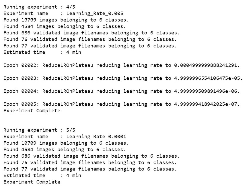

Result
From the above table, it is clear that Learning_Rate_0.0001 has the least validation loss. We will update our learning rate with this.
ktf.update_learning_rate(0.0001)
# Very important to reload post updates ktf.Reload()
b. Analyze Batch sizes
# Analysis Project Name
analysis_name = "analyse_batch_sizes_vgg16"# Batch sizes to explore
batch_sizes = [2, 4, 8, 12]# Note: We're using the same percent_data and num_epochs.
# "keep_all" - Keep all the sub experiments created
# "keep_none" - Delete all sub experiments createdanalysis_batches = ktf.Analyse_Batch_Sizes(analysis_name, batch_sizes, percent_data, num_epochs=epochs, state="keep_none")

Result
From the above table, it is clear that Batch_Size_12 has the least validation loss. We will update the model with this.
ktf.update_batch_size(12)# Very important to reload post updates
ktf.Reload()
c. Analyse Optimizers
# Analysis Project Name
analysis_name = "analyse_optimizers_vgg16"# Optimizers to explore
optimizers = ["sgd", "adam", "adagrad"]# "keep_all" - Keep all the sub experiments created
# "keep_non" - Delete all sub experiments createdanalysis_optimizers = ktf.Analyse_Optimizers(analysis_name, optimizers, percent_data, num_epochs=epochs, state="keep_none")

Result
From the above table, it is clear that we should go for Optimizer_adagrad since it has the least validation loss.
Summary of Hyperparameter Tuning Experiment
Here ends our Experiment, and now it’s time to switch on the Expert Mode to train our classifier using the above Hyperparameters.
Summary:
- Learning Rate — 0.0001
- Batch size — 12
- Optimizer — adagrad
1. Training from scratch: vgg16
Expert Mode
Let’s create another Experiment named expert_mode_vgg16 and train our classifier from scratch.
ktf = prototype(verbose=1)ktf.Prototype("Project-Zalando", "expert_mode_vgg16")ktf.Dataset_Params(dataset_path="/content/drive/My Drive/Data/zalando", split=0.8, input_size=224, batch_size=12, shuffle_data=True, num_processors=2)# Load the dataset
ktf.Dataset()ktf.Model_Params(model_name="vgg16", freeze_base_network=True, use_gpu=True, use_pretrained=True)ktf.Model()ktf.Training_Params(num_epochs=5, display_progress=True, display_progress_realtime=True, save_intermediate_models=True, intermediate_model_prefix="intermediate_model_", save_training_logs=True)# Update optimizer and learning rate
ktf.optimizer_adagrad(0.0001)ktf.loss_crossentropy()# Training
ktf.Train()
Output:

Validation
ktf = prototype(verbose=1);ktf.Prototype("Project-Zalando", "expert_mode_vgg16", eval_infer=True)# Just for example purposes, validating on the training set itself
ktf.Dataset_Params(dataset_path="/content/drive/My Drive/Data/zalando")ktf.Dataset()accuracy, class_based_accuracy = ktf.Evaluate()

Inference
Let’s see the Prediction on sample images.
ktf = prototype(verbose=1)ktf.Prototype("Project-Zalando", "expert_mode_vgg16", eval_infer=True)
The model is now loaded.
img_name = "/content/[email protected]"
predictions = ktf.Infer(img_name=img_name)#Display
from IPython.display import Image
Image(filename=img_name)

We’ve successfully completed training our classifier. Check the logs and models folder under this Experiment to see the model weights and other insights.
2. Training from scratch: mobilenet_v2
I have gone ahead and trained mobilenet_v2 from scratch in the same way to compare vgg16 and mobilenet_v2.
After the Experiment, the best hyperparameters for mobilenet_v2 are:
- Learning Rate — 0.0001
- Batch Size — 8
- Optimizer — adam
Expert Mode
ktf = prototype(verbose=1)
ktf.Prototype("Project-Zalando", "expert_mode_mobilenet_v2")ktf.Dataset_Params(dataset_path="/content/drive/My Drive/Data/zalando", split=0.8, input_size=224, batch_size=8, shuffle_data=True, num_processors=2)ktf.Dataset()ktf.Model_Params(model_name="mobilenet_v2", freeze_base_network=True, use_gpu=True, use_pretrained=True)ktf.Model()ktf.Training_Params(num_epochs=5, display_progress=True, display_progress_realtime=True, save_intermediate_models=True, intermediate_model_prefix="intermediate_model_", save_training_logs=True)ktf.optimizer_adam(0.0001)ktf.loss_crossentropy()ktf.Train()

Validation
ktf = prototype(verbose=1)
ktf.Prototype("Project-Zalando", "expert_mode_mobilenet_v2", eval_infer=True)# Just for example purposes, validating on the training set itself
ktf.Dataset_Params(dataset_path="/content/drive/My Drive/Data/zalando")ktf.Dataset()accuracy, class_based_accuracy = ktf.Evaluate()

Inference
ktf = prototype(verbose=1)ktf.Prototype("Project-Zalando", "expert_mode_mobilenet_v2", eval_infer=True)
The model is now loaded.
img_name = "/content/[email protected]"
predictions = ktf.Infer(img_name=img_name)#Display
from IPython.display import Image
Image(filename=img_name)

img_name = "/content/[email protected]"
predictions = ktf.Infer(img_name=img_name)#Display
from IPython.display import Image
Image(filename=img_name)

Comparing vgg16 and mobilenet_v2
I’ve used the same tutorial, which I mentioned previously, to compare these two experiments.
# Invoke the comparison class
# import monk_v1
from compare_prototype import compare# Create a project
ctf = compare(verbose=1)
ctf.Comparison("vgg-mobilenet-Comparison")ctf.Add_Experiment("Project-Zalando", "expert_mode_vgg16")
ctf.Add_Experiment("Project-Zalando", "expert_mode_mobilenet_v2")ctf.Generate_Statistics()
After the statistics are generated,
from IPython.display import ImageImage(filename="/content/drive/My Drive/Monk_v1/workspace/comparison/vgg-mobilenet-Comparison/train_accuracy.png")

from IPython.display import ImageImage(filename="/content/drive/My Drive/Monk_v1/workspace/comparison/vgg-mobilenet-Comparison/train_loss.png")

from IPython.display import ImageImage(filename="/content/drive/My Drive/Monk_v1/workspace/comparison/vgg-mobilenet-Comparison/val_accuracy.png")

from IPython.display import ImageImage(filename="/content/drive/My Drive/Monk_v1/workspace/comparison/vgg-mobilenet-Comparison/val_loss.png")

from IPython.display import ImageImage(filename="/content/drive/My Drive/Monk_v1/workspace/comparison/vgg-mobilenet-Comparison/stats_training_time.png")

from IPython.display import ImageImage(filename="/content/drive/My Drive/Monk_v1/workspace/comparison/vgg-mobilenet-Comparison/stats_best_val_acc.png")

Conclusion
From the above comparisons, it is clear that the model vgg16 performed better in every aspect.
There is a lot of room for improving the model’s accuracy by further tuning the hyperparameters. Please refer to Image Classification Zoo for more tutorials.
Tutorial available on GitHub. Please Clap or Share this article if it helped you learn something!
Join thousands of data leaders on the AI newsletter. Join over 80,000 subscribers and keep up to date with the latest developments in AI. From research to projects and ideas. If you are building an AI startup, an AI-related product, or a service, we invite you to consider becoming a sponsor.
Published via Towards AI
Related posts
Popular posts

 for 2021")


Updates

Recent Posts