How To Win Your NHL Pool Without Even Trying

Last Updated on January 17, 2021 by Editorial Team

Author(s): Yan Gobeil

Machine Learning

How I used machine learning to predict the number of points that a hockey player will score this year

With the new National Hockey League (NHL) season just around the corner, I received an unexpected invitation to participate in a pool with people from the blind hockey community. The idea is to pick a player in each of the 24 groups of six similar players to form your team. The winner is the person whose team gets the most points during the season. After trying to choose players for a couple of minutes, I started to wonder how hard it would be to train a machine learning model that helps me in this task. In this blog post, I share how I ended up building that model and using it to make my picks.

Collecting the data

The first step in every good machine learning project is to find some data. In my case, I had to find the player stats from a few of the previous NHL seasons. I was set in my mind that I would scrape NHL.com to get that data when I discovered that there is actually an API made by the NHL for that. It is extremely badly documented by the NHL but a random guy generously made incredible documentation with a surprising amount of detail, which can be found here. This is the tool that I ended up using to collect my data.

The strategy that I chose is to use data from the last 10 seasons and use the player stats from two consecutive seasons to predict the points scored in the following one. I will not detail all my code, which can be found in this colab notebook, but I will describe the main steps. I first used the standings endpoint of the NHL API to extract the list of ids of the teams that appeared in the NHL between the 2010–2011 and 2019–2020 seasons. I then used the teams endpoint to obtain the rosters of each of these teams for each of the seasons of interest. This was the list of players that I would consider.

The next step was to extract as much data as possible for these players. I had to use two different endpoints for that. The people endpoint gave me personal information like birthday, height and weight, and the stats extension of the same endpoint gave me access to the hockey stats like goals, assists and games played for each of the seasons played by the player. Stats about seasons played in other leagues are actually available so I had to make sure to pick only the NHL seasons, within my range of years. Here is an example of each of the URLs that I used to collect my data:

list of teams playing in the 2019-2020 season:
https://statsapi.web.nhl.com/api/v1/standings?season=20192020

List of players who played for the Pittsburgh Penguins (id=5) in 2019-2020:
https://statsapi.web.nhl.com/api/v1/teams/5/?expand=team.roster&season=20192020

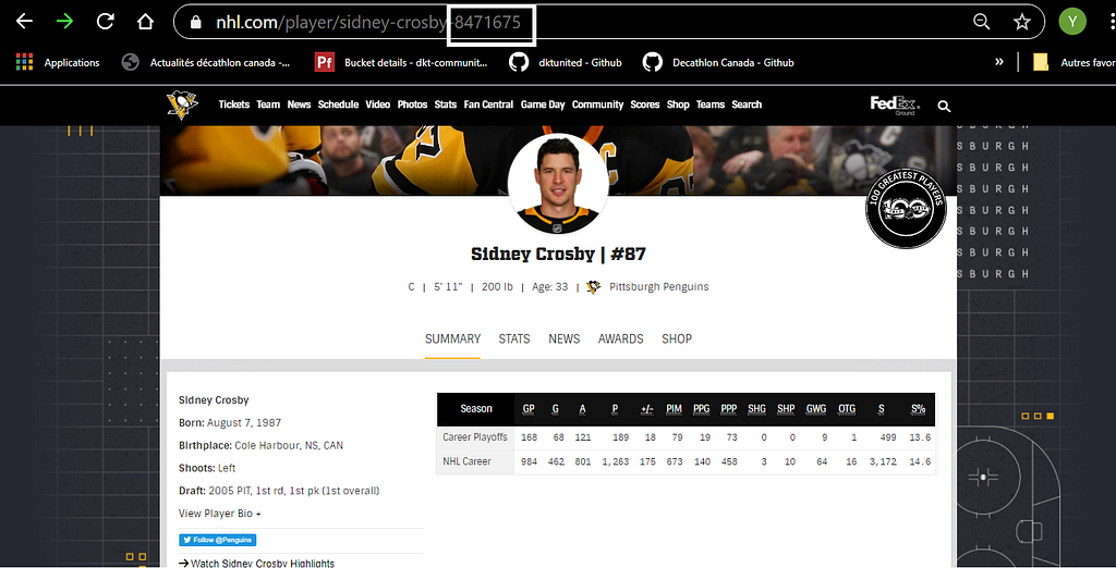
Personal information of Sidney Crosby (id=8471675):
https://statsapi.web.nhl.com/api/v1/people/8471675

Career stats of Sidney Crosby (id=8471675):
https://statsapi.web.nhl.com/api/v1/people/8471675/stats?stats=yearByYear

This strategy gave me stats for a total of 2115 players. Unfortunately a large number of these players have not played enough to be useful as training data so I had to reduce the list to only players who had played at least 3 seasons and 100 games during the decade. I also removed the goalies because they are totally different beasts from the rest of the players. This reduced the list to 1038 players.

The last step before jumping into modelling was to put the data into the format required for training, which is a list of pairs of consecutive seasons with their corresponding stats and the points scored in the following season, to be used as label. To try to make good predictions for second year players, who only have one year of history, I kept lines where one of the two seasons didn’t have any games played. This left me with 5105 lines of data.

Data preprocessing

I collected a lot of stats for each player and not necessarily all of them should be useful to predict the performance for next season. The data was also in a very raw format so I had to clean it up a lot. Here is the list of features that I ended up keeping and how they were processed:

• Height, converted to inches
• Weight in pounds
• Age as of the first season of the relevant triplet
• Position (L, R, C, D) encoded into four indicators
• Goals per game played, for each of the two seasons
• Points per game played, for each of the two seasons
• Hits per game played, for each of the two seasons
• Shots per game played, for each of the two seasons
• Penalty minutes per game played, for each of the two seasons
• Time on ice per game played, for each of the two seasons
• Fraction of 82 games played during each of the two seasons
• Plus/Minus total, for each of the two seasons

Since the number of points is extremelly related to the number of games played, I decided to predict the number of points per game instead for the third season of the triplet.

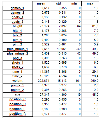
Even after all this data processing, there were still a few features that were not ideal. Indeed, it is known that machine learning algorithms work better when the features are small numbers between -1 and 1. This meant that I had to normalize (subtract mean and divide by standard deviation) the following features: height, weight, age, plus/minus and time on ice. It is extremelly important however to perform this normalization using the training data only to not inject information about the testing data into the model. This step was thus done after randomly splitting the full data into 85% for training and 15% for testing.

Building a model

Before jumping into complicated modelling, it is always a good idea to build the simplest predictor possible to use as benchmark. One idea for this setup was simply to use the points per game of the last season and assume that the player will keep the same production. Note that this is a regression task, so the losses and metrics used are not the same as when doing classification. In this case I chose Mean Squared Error (MSE) and Root Mean Squared Error (RMSE), which is simply MSE’s square root. Evaluating those metrics for the benchmark model on the test data gives:

MSE: 0.0323
RMSE: 0.180

This means that using this method, we were wrong by 0.18 points per game on average. It is not perfect for sure, but not too bad at the same time since it corresponds to 15 points on an 82-game season.

Next, the first model to always try when working on regression is Linear Regression, which I implemented using the sklearn library. After being fit to the training data, the model achieved the following performance on the test data:

MSE: 0.0243
RMSE: 0.156

These metrics are still not perfect, but they show a clear improvement over the simple benchmark.

Instead of playing around for hours with different sklearn models for regression, I jumped directly into Neural Networks, which I trained using the autokeras library for simplicity. I don’t recommend using autoML for every possible task since human expertise often beats it, but for a simple task like this one it was not worth wasting my time on manual optimization of neural network architectures and hyperparameters. To my surprise, I only got to improve the linear regression results by a tiny amount using neural networks. The best results that I achieved throughout all my tries were:

MSE: 0.0229
RMSE: 0.151

Analyzing the model

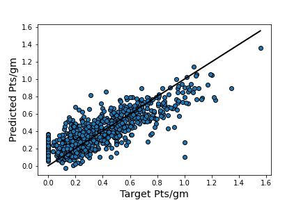
To summarize the model building part of the project, I ended up with two similar models that are wrong by around 12 points on average over the whole season. It is also interesting to see that predictions seem to underestimate the true values for better players and overestimate it for average players (see plot), but for my use case I only cared about comparing similar players, so this was not a huge problem.

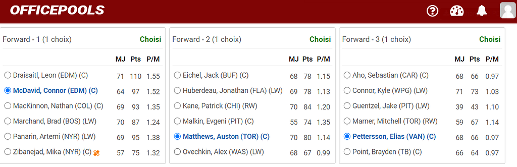
Now that I had my final model, it was time to make predictions for the 2020–2021 season in order to win my pool! After doing the same preprocessing on the data as before and using the trained linear regression model, here are the predictions for the first set of players that I had to choose from:

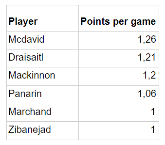
This means that I had to pick Connor Mcdavid, who was my choice anyway! For the curious readers, here is what the model predicted for the top 5 players of the season: Mcdavid, Draisaitl, Mackinnon, Pastrnak, Kucherov.

It is interesting to see that an unknown player like Morgan Geekie enterred the top 15, but this can be explained simply by the fact that he only has 2 games of experience in the NHL, so the model must have randomly guessed his future performance.

Improving the model?

I am somehow satisfied with the model that I built, but there is of course still plenty of room for improvement. There are many other factors that influence a player’s performance, like his teammates and linemates. It could also be useful to consider more than two seasons in the past and to collect more data overall. Perhaps more advanced stats could also be important in understanding a player’s potential as well.

Since I was in a rush (the season starts tonight…) I didn’t focus on improving the model as much as possible. I am still curious to see how the model will perform so I will post an update later in the season for those fo you who care 🙂

How To Win Your NHL Pool Without Even Trying was originally published in Towards AI on Medium, where people are continuing the conversation by highlighting and responding to this story.

Published via Towards AI