Graph Attention Networks Paper Explained With Illustration and PyTorch Implementation

Author(s): Ebrahim Pichka

Originally published on Towards AI.

A detailed and illustrated walkthrough of the “Graph Attention Networks” paper by Veličković et al. with the PyTorch implementation of the proposed model.

Introduction

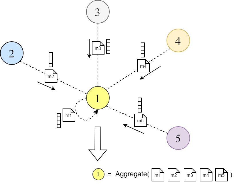
Graph neural networks (GNNs) are a powerful class of neural networks that operate on graph-structured data. They learn node representations (embeddings) by aggregating information from a node’s local neighborhood. This concept is known as ‘message passing’ in the graph representation learning literature.

Messages (embeddings) are passed between nodes in the graph through multiple layers of the GNN. Each node aggregates the messages from its neighbors to update its representation. This process is repeated across layers, allowing nodes to obtain representations that encode richer information about the graph. Some of the important variants of GNNs can are GraphSAGE [2], Graph Convolution Network [3], etc. You can explore more GNN variants here.

Graph Attention Networks (GAT) [1] are a special class of GNNs that were proposed to improve upon this message-passing scheme. They introduced a learnable attention mechanism that enables a node to decide which neighbor nodes are more important when aggregating messages from their local neighborhood by assigning a weight between each source and target node instead of aggregating information from all neighbors with equal weights.

Empirically, Graph Attention Networks have been shown to outperform many other GNN models on tasks such as node classification, link prediction, and graph classification. They demonstrated state-of-the-art performance on several benchmark graph datasets.

In this post, we will walk through the crucial part of the original “Graph Attention Networks” paper by Veličković et al. [1], explain these parts, and simultaneously implement the notions proposed in the paper using PyTorch framework to better grasp the intuition of the GAT method.

You can also access the full code used in this post, containing the training and validation code in this GitHub repository

Going Through the Paper

Section 1 — Introduction

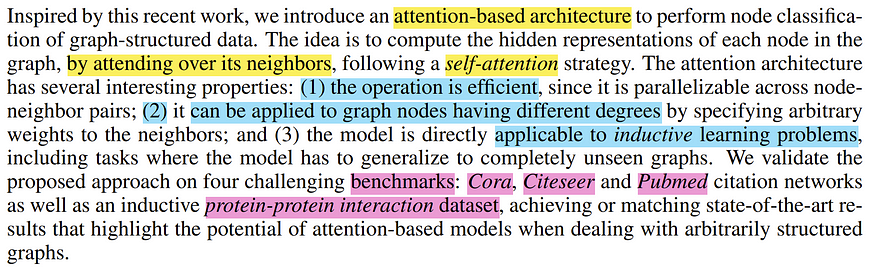
After broadly reviewing the existing methods in the graph representation learning literature in Section 1, “Introduction”, the Graph Attention Network (GAT) is introduced. The authors mention:

1. An overall view of the incorporated attention mechanism.
2. Three properties of GATs, namely efficient computation, general applicability to all nodes, and usability in inductive learning.
3. Benchmarks and Datasets on which they evaluated the GAT’s performance.

Then After comparing their approach to some existing methods and mentioning the general similarities and differences between them, they move forward to the next section of the paper.

Section 2 — GAT Architecture

In this section, which accounts for the main part of the paper, the Graph Attention Network architecture is laid out in detail. To move forward with the explanation, assume the proposed architecture performs on a graph with N nodes (V = {vᵢ}; i=1,…,N) and each node is represented with a vector hᵢ of F elements, With any arbitrary setting of edges existing between nodes.

The authors first start by characterizing a single Graph Attention Layer, and how it operates, which becomes the building blocks of a Graph Attention Network. In general, a single GAT layer is supposed to take a graph with its given node embeddings (representations) as input, propagate information to local neighbor nodes, and output an updated representation of nodes.

As highlighted above, to do so, first, they state that all the input node feature vectors (hᵢ) to the GA-layer are linearly transformed (i.e. multiplied by a weight matrix W), in PyTorch, it is generally done as follows:

import torch
from torch import nn

# in_features -> F and out_feature -> F'
in_features = ...
out_feature = ...

# instanciate the learnable weight matrix W (FxF')
W = nn.Parameter(torch.empty(size=(in_features, out_feature)))

# Initialize the weight matrix W
nn.init.xavier_normal_(W)

# multiply W and h (h is input features of all the nodes -> NxF matrix)
h_transformed = torch.mm(h, W)

Now having in mind that we obtained a transformed version of our input node features (embeddings), we jump a few steps forward to observe and understand what is our final objective in a GAT layer.

As described in the paper, at the end of a graph attention layer, for each node i, we need to obtain a new feature vector that is more structure- and context-aware from its neighborhood.

This is done by calculating a weighted sum of neighboring node features followed by a non-linear activation function σ. This weighted sum is also known as the ‘Aggregation Step’ in the general GNN layer operations, according to Graph ML literature.

These weights αᵢⱼ ∈ [0, 1] are learned and computed by an attention mechanism that denotes the importance of the neighbor j features for node i during message passing and aggregation.

Now let’s see how these attention weights αᵢⱼ are computed for each pair of node i and its neighbor j:

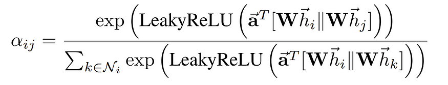
In short, attention weights αᵢⱼ are calculated as below

Where the eᵢⱼ are attention scores and the Softmax function is applied so that all the weights are in the [0, 1] interval and sum to 1.

The attention scores eᵢⱼ are now calculated between each node i and its neighbors j ∈ Nᵢ through the attention function a(…) as such:

Where U+007CU+007C denotes the concatenation of two transformed node embeddings, and a is a vector of learnable parameters (i.e., attention parameters) of the size 2 * F’ (twice the size of transformed embeddings).

And the (aᵀ) is the transpose of the vector a, resulting in the whole expression aᵀ [WhᵢU+007CU+007C Whⱼ] being the dot (inner) product between “a” and the concatenation of transformed embeddings.

The whole operation is illustrated below:

In PyTorch, to achieve these scores, we take a slightly different approach. Because it is more efficient to compute eᵢⱼ between all pairs of nodes and then select only those which represent existing edges between nodes. To calculate all eᵢⱼ:

# instanciate the learnable attention parameter vector `a`
a = nn.Parameter(torch.empty(size=(2 * out_feature, 1)))

# Initialize the parameter vector `a`
nn.init.xavier_normal_(a)

# we obtained `h_transformed` in the previous code snippet

# calculating the dot product of all node embeddings
# and first half the attention vector parameters (corresponding to neighbor messages)
source_scores = torch.matmul(h_transformed, self.a[:out_feature, :])

# calculating the dot product of all node embeddings
# and second half the attention vector parameters (corresponding to target node)
target_scores = torch.matmul(h_transformed, self.a[out_feature:, :])

# broadcast add 
e = source_scores + target_scores.T
e = self.leakyrelu(e)

The last part of the code snippet (# broadcast add) adds all the one-to-one source and target scores, resulting in an NxN matrix containing all the eᵢⱼ scores. (illustrated below)

So far, it’s like we assumed the graph is fully-connected and calculated the attention scores between all possible pair of nodes. To address this, after the LeakyReLU activation is applied to the attention scores, the attention scores are masked based on existing edges in the graph, meaning we only keep the scores that correspond to existing edges.

It can be done by assigning a large negative score (to approximate -∞) to elements in the scores matrix between nodes with non-existing edges so their corresponding attention weights become zero after softmax.

We can achieve this by using the adjacency matrix of the graph. The adjacency matrix is an NxN matrix with 1 at row i and column j if there is an edge between node i and j and 0 elsewhere. So we create the mask by assigning -∞ to zero elements of the adjacency matrix and assigning 0 elsewhere. And then, we add the mask to our scores matrix. and apply the softmax function across its rows.

connectivity_mask = -9e16 * torch.ones_like(e)
# adj_mat is the N by N adjacency matrix
e = torch.where(adj_mat > 0, e, connectivity_mask) # masked attention scores
 
# attention coefficients are computed as a softmax over the rows
# for each column j in the attention score matrix e
attention = F.softmax(e, dim=-1)

Finally, according to the paper, after obtaining the attention scores and masking them with the existing edges, we get the attention weights αᵢⱼ by performing softmax over the rows of the scores matrix.

And as discussed before, we calculate the weighted sum of the node embeddings:

# final node embeddings are computed as a weighted average of the features of its neighbors
h_prime = torch.matmul(attention, h_transformed)

Finally, the paper introduces the notion of multi-head attention, where the whole discussed operations are done through multiple parallel streams of operations, where the final result heads are either averaged or concatenated.

The multi-head attention and aggregation process is illustrated below:

To wrap up the implementation in a cleaner modular form (as a PyTorch module) and to incorporate the multi-head attention functionality, the whole Graph Attention Layer implementation is done as follows:

import torch
from torch import nn
import torch.nn.functional as F

################################
### GAT LAYER DEFINITION ###
################################

class GraphAttentionLayer(nn.Module):

 def __init__(self, in_features: int, out_features: int,
 n_heads: int, concat: bool = False, dropout: float = 0.4,
 leaky_relu_slope: float = 0.2):
 super(GraphAttentionLayer, self).__init__()

 self.n_heads = n_heads # Number of attention heads
 self.concat = concat # wether to concatenate the final attention heads
 self.dropout = dropout # Dropout rate

 if concat: # concatenating the attention heads
 self.out_features = out_features # Number of output features per node
 assert out_features % n_heads == 0 # Ensure that out_features is a multiple of n_heads
 self.n_hidden = out_features // n_heads
 else: # averaging output over the attention heads (Used in the main paper)
 self.n_hidden = out_features

 # A shared linear transformation, parametrized by a weight matrix W is applied to every node
 # Initialize the weight matrix W 
 self.W = nn.Parameter(torch.empty(size=(in_features, self.n_hidden * n_heads)))

 # Initialize the attention weights a
 self.a = nn.Parameter(torch.empty(size=(n_heads, 2 * self.n_hidden, 1)))

 self.leakyrelu = nn.LeakyReLU(leaky_relu_slope) # LeakyReLU activation function
 self.softmax = nn.Softmax(dim=1) # softmax activation function to the attention coefficients

 self.reset_parameters() # Reset the parameters


 def reset_parameters(self):

 nn.init.xavier_normal_(self.W)
 nn.init.xavier_normal_(self.a)

 def _get_attention_scores(self, h_transformed: torch.Tensor):
 
 source_scores = torch.matmul(h_transformed, self.a[:, :self.n_hidden, :])
 target_scores = torch.matmul(h_transformed, self.a[:, self.n_hidden:, :])

 # broadcast add 
 # (n_heads, n_nodes, 1) + (n_heads, 1, n_nodes) = (n_heads, n_nodes, n_nodes)
 e = source_scores + target_scores.mT
 return self.leakyrelu(e)

 def forward(self, h: torch.Tensor, adj_mat: torch.Tensor):

 n_nodes = h.shape[0]

 # Apply linear transformation to node feature -> W h
 # output shape (n_nodes, n_hidden * n_heads)
 h_transformed = torch.mm(h, self.W)
 h_transformed = F.dropout(h_transformed, self.dropout, training=self.training)

 # splitting the heads by reshaping the tensor and putting heads dim first
 # output shape (n_heads, n_nodes, n_hidden)
 h_transformed = h_transformed.view(n_nodes, self.n_heads, self.n_hidden).permute(1, 0, 2)
 
 # getting the attention scores
 # output shape (n_heads, n_nodes, n_nodes)
 e = self._get_attention_scores(h_transformed)

 # Set the attention score for non-existent edges to -9e15 (MASKING NON-EXISTENT EDGES)
 connectivity_mask = -9e16 * torch.ones_like(e)
 e = torch.where(adj_mat > 0, e, connectivity_mask) # masked attention scores
 
 # attention coefficients are computed as a softmax over the rows
 # for each column j in the attention score matrix e
 attention = F.softmax(e, dim=-1)
 attention = F.dropout(attention, self.dropout, training=self.training)

 # final node embeddings are computed as a weighted average of the features of its neighbors
 h_prime = torch.matmul(attention, h_transformed)

 # concatenating/averaging the attention heads
 # output shape (n_nodes, out_features)
 if self.concat:
 h_prime = h_prime.permute(1, 0, 2).contiguous().view(n_nodes, self.out_features)
 else:
 h_prime = h_prime.mean(dim=0)

 return h_prime

Next, the authors do a comparison between GATs and some of the other existing GNN methodologies/architectures. They argue that:

1. GATs are computationally more efficient than some existing methods due to being able to compute attention weights and perform the local aggregation in parallel.
2. GATs can assign different importance to neighbors of a node while aggregating messages which can enable a leap in model capacity and increase interpretability.
3. GAT does consider the complete neighborhood of nodes (does not require sampling from neighbors) and it does not assume any ordering within nodes.
4. GAT can be reformulated as a particular instance of MoNet (Monti et al., 2016) by setting the pseudo-coordinate function to be u(x, y) = f(x)U+007CU+007Cf(y), where f(x) represents (potentially MLP-transformed) features of node x and U+007CU+007C is concatenation; and the weight function to be wj(u) = softmax(MLP(u))

Section 3 — Evaluation

In the third section of the paper, first, the authors describe the benchmarks, datasets, and tasks on which the GAT is evaluated. Then they present the results of their evaluation of the model.

Transductive learning vs. Inductive learning
Datasets used as benchmarks in this paper are differentiated into two types of tasks, Transductive and Inductive.

• Inductive learning: It is a type of supervised learning task in which a model is trained only on a set of labeled training examples and the trained model is evaluated and tested on examples that were completely unobserved during training. It is the type of learning which is known as common supervised learning.
• Transductive learning: In this type of task, all the data, including training, validation, and test instances, are used during training. But in each phase, only the corresponding set of labels is accessed by the model. Meaning during training, the model is only trained using the loss that is resulted from the training instances and labels, but the test and validation features are used for the message passing. It is mostly because of the structural and contextual information existing in the examples.

Datasets
In the paper, four benchmark datasets are used to evaluate GATs, three of which correspond to transductive learning, and one other is used as an inductive learning task.

The transductive learning datasets, namely Cora, Citeseer, and Pubmed (Sen et al., 2008) datasets are all citation graphs in which nodes are published documents and edges (connections) are citations among them, and the node features are elements of a bag-of-words representation of a document. The inductive learning dataset is a protein-protein interaction (PPI) dataset containing graphs are different human tissues (Zitnik & Leskovec, 2017). Datasets are described more below:

Setup & Results

• For the three transductive tasks, the setting used for training is:
  They use 2 GAT layers — layer 1 uses
  – K = 8 attention heads
  – F’ = 8 output feature dim per head
  – ELU activation
  and for the second layer [Cora & Citeseer U+007C Pubmed]
  – [1 U+007C 8] attention head with C number of classes output dim
  – Softmax activation for classification probability output
  and for the overall network
  – Dropout with p = 0.6
  – L2 regularization with λ = [0.0005 U+007C 0.001]
• For the three transductive tasks, the setting used for training is:
  Three layers —
  – Layer 1 & 2: K = 4 U+007C F’ = 256 U+007C ELU
  – Layer 3: K = 6 U+007C F’ = C classes U+007C Sigmoid (multi-label)
  with no regularization and dropout

The first setting’s implementation in PyTorch is done below using the layer we defined earlier:

class GAT(nn.Module):

 def __init__(self,
 in_features,
 n_hidden,
 n_heads,
 num_classes,
 concat=False,
 dropout=0.4,
 leaky_relu_slope=0.2):

 super(GAT, self).__init__()

 # Define the Graph Attention layers
 self.gat1 = GraphAttentionLayer(
 in_features=in_features, out_features=n_hidden, n_heads=n_heads,
 concat=concat, dropout=dropout, leaky_relu_slope=leaky_relu_slope
 )
 
 self.gat2 = GraphAttentionLayer(
 in_features=n_hidden, out_features=num_classes, n_heads=1,
 concat=False, dropout=dropout, leaky_relu_slope=leaky_relu_slope
 )

 def forward(self, input_tensor: torch.Tensor , adj_mat: torch.Tensor):


 # Apply the first Graph Attention layer
 x = self.gat1(input_tensor, adj_mat)
 x = F.elu(x) # Apply ELU activation function to the output of the first layer

 # Apply the second Graph Attention layer
 x = self.gat2(x, adj_mat)

 return F.softmax(x, dim=1) # Apply softmax activation function

After testing, the authors report the following performance for the four benchmarks showing the comparable results of GATs compared to existing GNN methods.

Conclusion

To conclude, in this blog post, I tried to take a detailed and easy-to-follow approach in explaining the “Graph Attention Networks” paper by Veličković et al. by using illustrations to help readers understand the main ideas behind these networks and why they are important for working with complex graph-structured data (e.g., social networks or molecules). Additionally, the post includes a practical implementation of the model using PyTorch, a popular programming framework. By going through the blog post and trying out the code, I hope readers can gain a solid understanding of how GATs work and how they can be applied in real-world scenarios. I hope this post has been helpful and encouraging to explore this exciting area of research further.

Plus, you can access the full code used in this post, containing the training and validation code in this GitHub repository.

I’d be happy to hear any thoughts or any suggestions/changes on the post.

References

[1] — Graph Attention Networks (2017), Petar Veličković, Guillem Cucurull, Arantxa Casanova, Adriana Romero, Pietro Liò, Yoshua Bengio. arXiv:1710.10903v3

[2] — Inductive Representation Learning on Large Graphs (2017), William L. Hamilton, Rex Ying, Jure Leskovec. arXiv:1706.02216v4

[3] — Semi-Supervised Classification with Graph Convolutional Networks (2016), Thomas N. Kipf, Max Welling. arXiv:1609.02907v4

Join thousands of data leaders on the AI newsletter. Join over 80,000 subscribers and keep up to date with the latest developments in AI. From research to projects and ideas. If you are building an AI startup, an AI-related product, or a service, we invite you to consider becoming a sponsor.

Published via Towards AI