


From Bits to Biology #1: Using LCS Algorithm for Global Sequence Alignment in Computational Biology
Last Updated on July 19, 2023 by Editorial Team
Author(s): Suyang Li
Originally published on Towards AI.
A step-by-step analysis of the Longest Common Subsequence problem and the Sequence Alignment problem with an explanation of their solutions highlighting their similarities and differences
Introduction
Welcome! You’ve found the first entry in my From Bits to Biology series, where I explore the connections between general algorithms you may find in a computer science class and computational biology/bioinformatics to make them more intuitive and accessible to those without formal biology training. It took me some time to be convinced you don’t necessarily need a formal biology background to make meaningful contributions in computational biology — an incredibly fascinating field — and I hope I’ll convince you to give it a try if you are in a similar boat 🙂
In this article, we are looking at Sequence Alignment, one of the most fundamental problems in computational biology. Alignment of DNA, RNA, and protein sequences has a variety of profound implications, including understanding evolutionary relationships, progressing functional annotation, identifying mutations, and advancing drug design and precision medicine.
Table of contents
- Longest Common Subsequence (LCS)
– LCS Overview
– LCS Dynamic programming solution
– LCS Python implementation - Global Sequence Alignment (GSA)
– GSA Overview
– Scoring Sytems
– GSA Dynamic programming solution
– GSA Python implementation - LCS vs. Global Sequence Alignment: Similarities and Differences
– Summary table
Longest Common Subsequence (LCS) Problem
Longest Common Subsequence (LCS) is a classic computer science problem that identifies the longest subsequence among all the valid subsequences shared between 2 or more input sequences.
Let’s clarify the LCS problem statement by first noting an important distinction between a subsequence and a substring. Take the sequence "ABCDE":
- A substring consists of contiguous characters in their original order. For example, valid substrings include
"ABC",“CD”, etc, but not“ABDE”or“CBA”. - A subsequence, on the other hand, does not have to be contiguous but must also be in the original order. For example, valid subsequences include
“AC”and“BFG”.
The LCS, then, is the longest among all the possible subsequences between 2 or more sequences. Here’s a quick example:

In practice, LCS has many applications involving much larger textual data, such as plagiarism detection¹ or Unix’s diff command, necessitating an efficient and reliable, scalable algorithmic solution.
Formalizing the LCS solution
Here’s a refresher on the 3-step dynamic programming solution to LCS:
- Initialization (create an m × n matrix, where m and n are the lengths of sequence 1 and sequences 2).
- Fill out the matrix according to the recurrence formula given below.
- Traceback to find the LCS as well as its length.
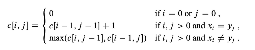
Consider the inputs “LONGEST” and “STONE”. Based on the recurrence relation given above, we fill out the DP matrix and then traceback as follows:
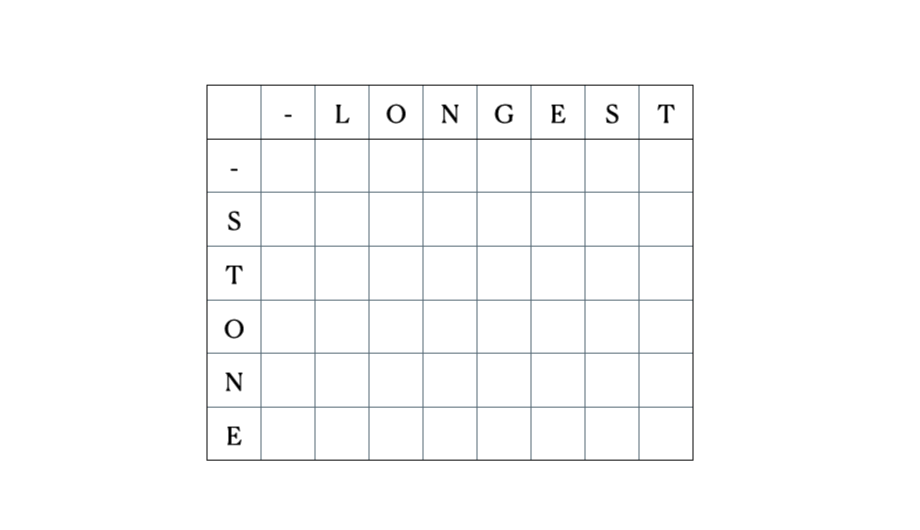
This is the full DP table:
This translates into the Python implementation below:
# Longest Common Subsequence
def lcs(seq1, seq2):
 m = len(seq1)
 n = len(seq2)

 # Construct dp table
 table = [[0 for x in range(n+1)] for x in range(m+1)]
 # Fill table based on recursive formula (15.9) from CLRS
 for i in range(m+1):
 for j in range(n+1):
 if i == 0 or j == 0: # case 1
 table[i][j] = 0
 elif seq1[i-1] == seq2[j-1]: # case 2
 table[i][j] = table[i-1][j-1] + 1
 else: # case 3
 table[i][j] = max(table[i-1][j], table[i][j-1])

 # Begin traceback from the bottom-rightmost cell
 index = table[m][n]
 lcs = [""] * (index+1)
 lcs[index] = ""

 i = m
 j = n
 while i > 0 and j > 0:
 if seq1[i-1] == seq2[j-1]: # add matching characters to LCS
 lcs[index-1] = seq1[i-1]
 i -= 1
 j -= 1
 index -= 1
 elif table[i-1][j] > table[i][j-1]:
 i -= 1
 else:
 j -= 1

 # Printing the longest common subsequence and its length
 print("Sequence 1: " + seq1 + "\nSequence 2: " + seq2)
 print("LCS: " + lcs + ", length: " + str(len(lcs)))
Example usage:
seq1 = 'STONE'
seq2 = 'LONGEST'
lcs(seq1, seq2)
Output:
Sequence 1: STONE
Sequence 2: LONGEST
LCS: ONE, length: 3
Now, let’s take a look at how this algorithm is used in the… ↓
(Global) Sequence Alignment Problem
Why do we want to align DNA/RNA/protein sequences?
In intuitive terms, aligning two sequences is a task of locating identical segments between the two sequences, serving the ultimate goal of assessing the level of similarity between them. Relatively straightforward in concept, this task has always been quite intricate in practice because of the uncountable changes that could happen to DNA and protein sequences through evolution. Specifically, common examples of these changes include:
- Point mutation, through insertion, deletion, or substitution:
– Insertion example: AAA → ACAA
– Deletion example: AAA → AA
– Substitution example: AAA → AGA - Fusion of sequences or segments from different genes
These unintended changes can introduce ambiguities and differences that mask our understanding of a given sequence. This is where we use alignment techniques to assess the similarity between sequences and infer characteristics such as homology.
How do we align sequences?
Because of these evolutionary changes, and because of the nature of biological sequence comparisons, unlike in LCS where we simply discard the “unmatchable” elements and only keep the common segment, in global sequence alignment, we must align all characters, which means alignments often involve 3 components:
- Matches, denoted by
U+007Cbetween the matching bases - Mismatches, denoted by blank spaces between the mismatched bases
- Gap insertions, denoted by dashes
—
Here’s an example. Suppose we have two DNA sequences “ACCCTG” and “ACCTGC”. There are a number of ways to match them base-to-base, taking into consideration the 3 operations we talked about earlier:
We could align them without any gap insertions:
ACCCTGT
U+007CU+007CU+007C U+007C
ACCTGCT
This alignment has 0 gap insertions, 3 matches, followed by 3 mismatches, and then 1 match at the end.
Or we could allow gap insertions in exchange for more matches:
ACCCTG-T
U+007CU+007CU+007C U+007CU+007C U+007C
ACC-TGCT
This alignment has 6 total matches, 2 gaps, and 0 mismatches (we don’t count a base-gap pair as a mismatch, since a gap penalty already comes with the gap insertion).
Or, if we really wished, we could also align them this way, which yields only 1 total match:
-ACC-CT-GT
 U+007C
ACCTG-CT--
Between any pair of sequences, there are almost always infinite ways to generate technically correct alignments as we saw just now. Some of them will be quite obviously worse than others, but there will be a few “approximately equally good” ones, such as options 1 and 2 above.
So, how do we evaluate the quality of each alignment, choose the optimal alignment, and break ties if we need to?
Scoring schemes
1. ACCCTGT 2. ACCCTG-T 3. -ACC-CTGT
 U+007CU+007CU+007C U+007C U+007CU+007CU+007C U+007CU+007C U+007C U+007C
 ACCTGCT ACC-TGCT ACCTG-CT-
In the example we saw above, each alignment involves a different combination of numbers of matches, mismatches, and gaps.
Unlike the LCS problem where a subsequence is only evaluated by its length — the longer the better — , in sequence alignment, we often measure the quality of an alignment by defining a quantitative scoring system that encompasses the 3 key components of each base-to-base pairing:
- Match reward: the score added to the overall alignment score whenever there is a base-to-base match pair in our sequence.
- Gap penalty: the penalty value subtracted from the overall alignment score each time we introduce a gap.
- Mismatch penalty: the penalty value subtracted from the overall alignment score each time we have a mismatch.
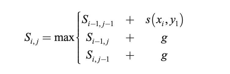
How do we formalize this as an algorithm?
The algorithmic solution significantly overlaps with the LCS solution in structure. It’s also a 3-step process, known as the Needleman-Wunsch algorithm:
- Initialization (create an m × n matrix, where m and n are the lengths of sequence 1 and sequences 2)
- Fill out the matrix according to the recursive formula given below
- Traceback to find the optimal alignment as well as its length
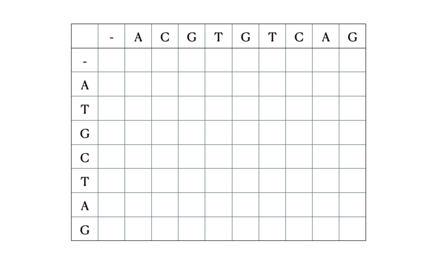
Before we get to the mathematical and Python formulation of the solution, here’s a quick illustration of the process with the sequences “ACGTGTCAG” and “ATGCTAG”:
Python solution
Let’s implement the Python solution using a class, GlobalSeqAlign, which handles both filling out the matrix as well as the traceback.
First, we construct an object containing the 5 pieces of key information: sequence 1, sequence 2, match score, mismatch penalty, and gap penalty.
class globalSeqAlign:
 def __init__(self, s1, s2, M, m, g):
 self.s1 = s1
 self.s2 = s2
 self.M = M
 self.m = m
 self.g = g
Then, we define a helper function that retrieves the score between two bases depending on whether they’re a match, mismatch, or base-gap pair:
 def base_pair_score(self, char1, char2):
 if char1 == char2:
 return self.M
 elif char1 == '-' or char2 == '-':
 return self.g
 else:
 return self.m
Now, we define a function very similar to the LCS function we saw earlier, which uses a m × n matrix, fills it according to the recursive formula, and then traces back to return the optimal alignment that maximizes the total score:
def optimal_alignment(self, s1, s2):
 m = len(s1)
 n = len(s2)
 score = [[0 for x in range(n+1)] for x in range(m+1)]

 # Calculate score table
 for i in range(m+1): # Initialize with 0s
 score[i][0] = self.g * i
 for j in range(n+1): # Initialize with 0s
 score[0][j] = self.g * j
 for i in range(1, m+1): # Fill remaining cells based on recursive formula above
 for j in range(1, n+1):
 match = score[i-1][j-1] + self.base_pair_score(s1[j-1], s2[i-1])
 delete = score[i-1][j] + self.g
 insert = score[i][j-1] + self.g
 score[i][j] = max(match, delete, insert)

 # Traceback, beginning from bottom-right cell
 align1 = ""
 align2 = ""
 i = m
 j = n

 while i > 0 and j > 0:
 score_curr = score[i][j]
 score_diag = score[i-1][j-1]
 score_up = score[i][j-1]
 score_left = score[i-1][j]

 if score_curr == score_diag + self.base_pair_score(s1[j-1], s2[i-1]): # match
 align1 += s1[j-1]
 align2 += s2[i-1]
 i -= 1
 j -= 1
 elif score_curr == score_up + self.g: # upward
 align1 += s1[j-1]
 align2 += '-'
 j -= 1
 elif score_curr == score_left + self.g: # leftward
 align1 += '-'
 align2 += s2[i-1]
 i -= 1
 while j > 0:
 align1 += s1[j-1]
 align2 += '-'
 j -= 1
 while i > 0:
 align1 += '-'
 align2 += s2[i-1]
 i -= 1

 return(align1[::-1], align2[::-1]) # Reverse order
Once we have the optimal alignment, we can then proceed with the analysis quantifying how well the sequences match.
Quantifying similarity: percentage similarity
One of the simplest ways to measure the “level of similarity” is through percentage similarity. We take the optimal alignment, look at its length, and divide it by the total length of the matched regions.
For example:
Seq 1: ACACAGTCAT
 U+007CU+007CU+007CU+007C U+007CU+007CU+007CU+007CU+007C
Seq 2: ACACTGTCAT
There are 9 matches out of the 10 total pairs, which yields a 90% similarity. There are many other interesting ways to analyze the quality of an alignment, but the underlying mechanism of sequence alignment remains the same.
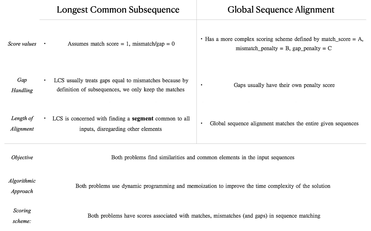
LCS & Global Sequence Alignment Comparison
Now that we have walked through both problems and their solutions in detail, let’s look at LCS and global sequence alignment side by side.
Similarities
- Objective: both problems find and maximize the similarities and common elements in the input sequences.
- Algorithmic approach: both problems can be solved using dynamic programming, which involves a DP matrix/table, filling out the matrix, and tracing back to produce the sequences/alignments.
- Scoring scheme: both problems have scores associated with matches, mismatches (and gaps) in sequence matching. These scores are explicitly and implicitly used in the algorithm to retrieve the optimal subsequence/alignment.
Differences
- Scoring systems:
– LCS automatically adopts a scoring scheme of match score = 1, mismatch/gap = 0;
– Global sequence alignment has a more complex scoring scheme defined by match score = A, mismatch penalty = B, gap penalty = C. - Gap Handling:
– LCS usually treats gaps equal to mismatches because by definition of subsequences, we only keep the matches;
– Global sequence alignment usually assigns gaps penalty score, different from the mismatch penalty if there is a preference for mismatch/gap. - Length of Alignment:
– LCS is concerned with finding a segment common to all inputs, disregarding the elements that are not part of this segment;
– Global sequence alignment matches the entire given sequences, even if it means inserting gaps if the input sequences differ in length.
Here’s a summary table of the points above:
Conclusion
Thanks for sticking with me this far U+1F63C! In this article, we focused on one specific dynamic programming problem — The longest Common Subsequence — and did a side-by-side comparison with its application in computational biology for Sequence Alignment.
Later in this series, we’ll also be looking at other topics, such as Hidden Markov Models, Gaussian Mixture Models, and Classification algorithms, and how they solve specific problems in computation biology. See you soon & Happy coding U+270CU+1F3FC!
[1] Baba, K., Nakatoh, T., & Minami, T. (2017). Plagiarism detection using document similarity based on distributed representation. Procedia Computer Science, 111, 382–387. https://doi.org/10.1016/j.procs.2017.06.038
[2] Cormen, T. H. (Ed.). (2009). Introduction to algorithms (3rd ed). MIT Press.
[3] Zvelebil, M. J., & Baum, J. O. (2008). Understanding bioinformatics. Garland Science.
Join thousands of data leaders on the AI newsletter. Join over 80,000 subscribers and keep up to date with the latest developments in AI. From research to projects and ideas. If you are building an AI startup, an AI-related product, or a service, we invite you to consider becoming a sponsor.
Published via Towards AI
Related posts


Popular posts

 for 2021")


Updates

Recent Posts


