


![Features in Image [Part -2]](https://miro.medium.com/v2/resize:fit:625/1*ELEtgIoW6AbMuQgGSSyIQA.gif "Features in Image [Part -2]")
Features in Image [Part -2]
Last Updated on July 24, 2023 by Editorial Team
Author(s): Akula Hemanth Kumar
Originally published on Towards AI.
Making computer vision easy with Monk, low code Deep Learning tool and a unified wrapper for Computer Vision.
Feature extraction and visualization using OpenCV and PIL
Level A features
HoG features
- Histogram of gradients.
- Used for Object Detection.
Steps
- Find gradients in both x and y directions
- Bin gradients into a histogram using the gradient magnitude and direction.
Hog features are sensitive to the rotation of objects in images.
Implementing Hog features using Skimage
Output
(322218,)


Daisy Features
- Upgraded HOG features
- Create a dense feature vector that is not suited for visualization.
Process
- T Block -> Calculate gradients or histogram of gradients
- S Block ->Combine T-block features using Gaussian weighted addition(profiles)
- N Block -> Normalize the added features(bring everything between 0–1)
- D Block -> Reduce dimensions of features (PCA algorithm)
- Q Block -> Compress features for storage purposes
Implementing Daisy Features using Sklearn
Output
(2, 3, 153)


GLCM Features
- Gray Level Covariance Matrix.
- Calculate the overall average for a degree of correlation between pairs of pixels in different aspects( in terms of homogeneity, uniformity)
- Gray -level co-occurrence matrix(GLCM)by calculating how often a pixel with the intensity (gray-level) value i occurs in a specific spatial relationship to a pixel with the value j.

Implementing GLCM features using Skimage

HAAR Features
- Used in object recognition.
Rectangular Haar-like Features
- A difference of the sum of the pixels of areas inside the rectangle.
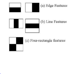
- Each feature is a single value obtained by the subtracted sum of pixels under the white rectangle from the sum of pixels under the black rectangle.
'''
Source:
https://scikitimage.org/docs/dev/auto_examples/features_detection/plot_haar.html
''' # Haar like feature Descriptors
import numpy as np
import matplotlib.pyplot as plt
import skimage.feature
from skimage.feature import haar_like_feature_coord, draw_haar_like_feature
images = [np.zeros((2, 2)), np.zeros((2, 2)),np.zeros((3, 3)), np.zeros((3, 3)),np.zeros((2, 2))]
feature_types = ['type-2-x', 'type-2-y','type-3-x', 'type-3-y', 'type-4']
fig, axs = plt.subplots(3, 2)
for ax, img, feat_t in zip(np.ravel(axs), images, feature_types):
 coord, _ = haar_like_feature_coord(img.shape[0],
 img.shape[1],
 feat_t)
 haar_feature = draw_haar_like_feature(img, 0, 0, img.shape[0],img.shape[1],coord,max_n_features=1, random_state=0)
 ax.imshow(haar_feature)
 ax.set_title(feat_t)
 ax.set_xticks([])
 ax.set_yticks([]) fig.suptitle('The different Haar-like feature descriptors') plt.axis('off')
plt.show()

LBP Features
- Local Binary Pattern
Elements
- LBP Thresholding
- Feature Summation

import numpy as np
import skimage
import skimage.feature
import cv2
from matplotlib import pyplot as plt
img = cv2.imread("imgs/chapter9/plant.jpg", 0);
#img = cv2.resize(img, (img.shape[0]//4,img.shape[1]//4));

output = skimage.feature.local_binary_pattern(img, 3, 8, method='default')
print(features.shape);

# Rescale histogram for better display
#output = skimage.exposure.rescale_intensity(output, in_range=(0, 10))


f = plt.figure(figsize=(15,15))
f.add_subplot(2, 1, 1).set_title('Original Image');
plt.imshow(img, cmap="gray")
f.add_subplot(2, 1, 2).set_title('Features');
plt.imshow(output);
plt.show()
Output
(2, 3, 153)


Blobs as features
- Blob detection methods are aimed at detecting regions in a digital image that differ in properties, such as brightness or color, compared to surrounding regions.
- Informally, a blob is a region of an image in which some properties are constant or approximately constant, all the points in a blob can be considered in some sense to be similar to each other.

Blobs using Skimage
import numpy as np
import skimage
import skimage.feature
import cv2
import math
from matplotlib import pyplot as plt

img = cv2.imread("imgs/chapter9/shape.jpg", 0)
#img = skimage.data.hubble_deep_field()[0:500, 0:500]
#image_gray = skimage.color.rgb2gray(image)

blobs = skimage.feature.blob_dog(img, max_sigma=5, threshold=0.05)

blobs[:, 2] = blobs[:, 2]
print(blobs.shape)

for y , x, r in blobs:
 cv2.circle(img,(int(x), int(y)), int(r), (0,255,0), 1)


f = plt.figure(figsize=(15,15))
f.add_subplot(2, 1, 1).set_title('Original Image');
plt.imshow(img, cmap="gray")
plt.show()
Output
(91, 3)

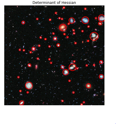
Using blobs to detect deep-space galaxies
'''
Source:
https://scikitimage.org/docs/dev/auto_examples/features_detection/plot_blob.html'''from math import sqrt
from skimage import data
from skimage.feature import blob_dog, blob_log, blob_doh
from skimage.color import rgb2gray

import matplotlib.pyplot as plt


image = data.hubble_deep_field()[0:500, 0:500]
image_gray = rgb2gray(image)

blobs_log = blob_log(image_gray, max_sigma=30, num_sigma=10, threshold=.1)

# Compute radii in the 3rd column.
blobs_log[:, 2] = blobs_log[:, 2] * sqrt(2)

blobs_dog = blob_dog(image_gray, max_sigma=30, threshold=.1)
blobs_dog[:, 2] = blobs_dog[:, 2] * sqrt(2)

blobs_doh = blob_doh(image_gray, max_sigma=30, threshold=.01)

blobs_list = [blobs_log, blobs_dog, blobs_doh]
colors = ['yellow', 'lime', 'red']
titles = ['Laplacian of Gaussian', 'Difference of Gaussian',
 'Determinant of Hessian']
sequence = zip(blobs_list, colors, titles)

fig, axes = plt.subplots(3, 1, figsize=(15, 15), sharex=True, sharey=True)
ax = axes.ravel()
for idx, (blobs, color, title) in enumerate(sequence):
 ax[idx].set_title(title)
 ax[idx].imshow(image, interpolation='nearest')
 for blob in blobs:
 y, x, r = blob
 c = plt.Circle((x, y), r, color=color, linewidth=2, fill=False)
 ax[idx].add_patch(c)
 ax[idx].set_axis_off()

plt.tight_layout()
plt.show()


Level B features
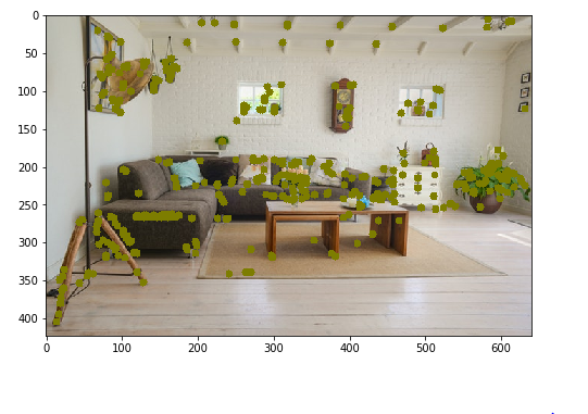
SIFT Features
- Scale Invariant Feature Transform.
- Patented in Canada by the University of British Columbia.
These features are:
- Scale-invariant
- Rotation invariant
- illumination invariant
- Viewpoint invariant
SIFT Steps
- Constructing a scale space -Pyramid generation
- LoG Approximation-laplacian of Gaussian features and gradients.
- Find key points- maxima and minima in the difference of Gaussian image.
- Eliminate bad keypoint.
- Assign an orientation to the key points.
- Generate final SIFT features- one more representation is generated for scale and rotation invariance.
Implementing SIFT features using OpenCV
'''
NOTE: Patented work. Cannot be used for commercial purposes1.pip install opencv-contrib-python==3.4.2.16
2.pip install opencv-python==3.4.2.16
'''
import numpy as np
import cv2
print(cv2.__version__)
from matplotlib import pyplot as plt
img = cv2.imread("imgs/chapter9/indoor.jpg", 1);

gray = cv2.cvtColor(img,cv2.COLOR_BGR2GRAY)

sift = cv2.xfeatures2d.SIFT_create()
keypoints, descriptors = sift.detectAndCompute(gray, None)


for i in keypoints:
 x,y = int(i.pt[0]), int(i.pt[1])
 cv2.circle(img,(x,y), 5,(0, 125, 125),-1)

plt.figure(figsize=(8, 8))
plt.imshow(img[:,:,::-1]);
plt.show()

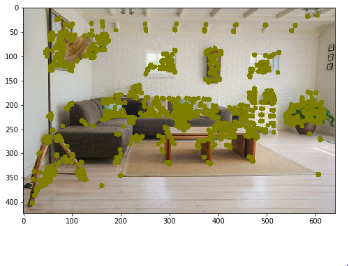
CenSurE Features
- Center Surround Extremes for Realtime Feature Detection.
- Outperforms many other keypoint detectors and feature extractors.
These features are
- Scale-invariant
- Rotation invariant
- Illumination invariant
- Viewpoint Invariant
Implementing CENSURE features using Skimage
import numpy as np
import cv2
import skimage.feature
from matplotlib import pyplot as plt
img = cv2.imread("imgs/chapter9/indoor.jpg", 1);

gray = cv2.cvtColor(img,cv2.COLOR_BGR2GRAY)

detector = skimage.feature.CENSURE(min_scale=1, max_scale=7, mode='Star',
 non_max_threshold=0.05, line_threshold=10)

detector.detect(gray)

for i in detector.keypoints:
 x,y = int(i[1]), int(i[0])
 cv2.circle(img,(x,y), 5,(0, 125, 125),-1)

plt.figure(figsize=(8, 8))
plt.imshow(img[:,:,::-1]);
plt.show()
SURF Features
- Speeded Up Robust Features.
- A patented local feature detector and descriptor.
- The standard version of SURF is several faster than SIFT.
SURF uses these algorithms
- Integer approximation of the determinant of Hessian blob detector.
- Sum of the Haar wavelet response
- Multi-resolution pyramid technique.
These features are
- Scale-invariant
- Rotation invariant
- Viewpoint invariant.
'''
NOTE: Patented work. Cannot be used for commercial purposes

1.pip install opencv-contrib-python==3.4.2.16
2.pip install opencv-python==3.4.2.16
'''import numpy as np
import cv2
from matplotlib import pyplot as plt
img = cv2.imread("imgs/chapter9/indoor.jpg", 1);

gray = cv2.cvtColor(img,cv2.COLOR_BGR2GRAY)

surf = cv2.xfeatures2d.SURF_create(1000)
keypoints, descriptors = surf.detectAndCompute(gray, None)


for i in keypoints:
 x,y = int(i.pt[0]), int(i.pt[1])
 cv2.circle(img,(x,y), 5,(0, 125, 125),-1)

plt.figure(figsize=(8, 8))
plt.imshow(img[:,:,::-1]);
plt.show()

BRIEF Features
- Binary Robust Independent Elementary Features.
- Outperforms other fast descriptors such as SURF and SIFT in terms of speed and terms of recognition rate in many cases.
Steps
- Image smoothing using gaussian kernels.
- Converting to Binary feature vector.
Implementing BRIEF features using OpenCV
import numpy as np
import cv2
from matplotlib import pyplot as plt
img = cv2.imread("imgs/chapter9/indoor.jpg", 1);

gray = cv2.cvtColor(img,cv2.COLOR_BGR2GRAY)

# Initiate FAST detector
star = cv2.xfeatures2d.StarDetector_create()
kp = star.detect(gray,None)

brief = cv2.xfeatures2d.BriefDescriptorExtractor_create()
keypoints, descriptors = brief.compute(gray, kp)


for i in keypoints:
 x,y = int(i.pt[0]), int(i.pt[1])
 cv2.circle(img,(x,y), 5,(0, 125, 125),-1)

plt.figure(figsize=(8, 8))
plt.imshow(img[:,:,::-1]);
plt.show()

BRISK Features
Binary Robust Independent Elementary Features.
Composed out of three parts
- A sampling pattern: where to sample points in the around the descriptor

- Orientation compensation: some mechanism to the orientation of the keypoint and rotate.
- Sampling pairs: which pairs to compare when building the final descriptor.
import numpy as np
import cv2
from matplotlib import pyplot as plt
img = cv2.imread("imgs/chapter9/indoor.jpg", 1);

gray = cv2.cvtColor(img,cv2.COLOR_BGR2GRAY)

brisk = cv2.BRISK_create()
keypoints, descriptors = brisk.detectAndCompute(gray, None)

for i in keypoints:
 x,y = int(i.pt[0]), int(i.pt[1])
 cv2.circle(img,(x,y), 5,(0, 125, 125),-1)

plt.figure(figsize=(8, 8))
plt.imshow(img[:,:,::-1]);
plt.show()
KAZE and Accelerated-KAZE features
KAZE Features using OpenCV
import numpy as np
import cv2
from matplotlib import pyplot as plt
img = cv2.imread("imgs/chapter9/indoor.jpg", 1);

gray = cv2.cvtColor(img,cv2.COLOR_BGR2GRAY)

kaze = cv2.KAZE_create()
keypoints, descriptors = kaze.detectAndCompute(gray, None)

for i in keypoints:
 x,y = int(i.pt[0]), int(i.pt[1])
 cv2.circle(img,(x,y), 5,(0, 125, 125),-1)

plt.figure(figsize=(8, 8))
plt.imshow(img[:,:,::-1]);
plt.show()

AKAZE Features
AKAZE Features using OpenCV
import numpy as np
import cv2
from matplotlib import pyplot as plt
img = cv2.imread("imgs/chapter9/indoor.jpg", 1);

gray = cv2.cvtColor(img,cv2.COLOR_BGR2GRAY)

akaze = cv2.AKAZE_create()
keypoints, descriptors = akaze.detectAndCompute(gray, None)

for i in keypoints:
 x,y = int(i.pt[0]), int(i.pt[1])
 cv2.circle(img,(x,y), 5,(0, 125, 125),-1)

plt.figure(figsize=(8, 8))
plt.imshow(img[:,:,::-1]);
plt.show()

ORB Features
Oriented Fast and Robust BRIEF Features
Orb Features using OpenCV
import numpy as np
import cv2
from matplotlib import pyplot as plt
img = cv2.imread("imgs/chapter9/indoor.jpg", 1)

gray = cv2.cvtColor(img,cv2.COLOR_BGR2GRAY)

orb = cv2.ORB_create(500)
keypoints, descriptors = orb.detectAndCompute(gray, None)

for i in keypoints:
 x,y = int(i.pt[0]), int(i.pt[1])
 cv2.circle(img,(x,y), 5,(0, 125, 125),-1)

plt.figure(figsize=(8, 8))
plt.imshow(img[:,:,::-1])
plt.show()

Feature matching
- Done to recognize similar features in multiple images.
- Used for object detection.
Methods
- Brute-Force
Matching every feature in image-1 against each feature in image-2
2. FLANN based matching
- Fast library for Approximate Nearest Neighbors.
- It contains a collection of algorithms optimized for fast nearest neighbor search in large datasets and for high dimensional features.
Feature Matching using OpenCV
'''
Using Brute-Force matching
'''
import numpy as np
import cv2
from matplotlib import pyplot as plt

orb = cv2.ORB_create(500)

img1 = cv2.imread("imgs/chapter9/indoor_lamp.jpg", 1);
img1 = cv2.resize(img1, (256, 256));
gray1 = cv2.cvtColor(img1,cv2.COLOR_BGR2GRAY);

img2 = cv2.imread("imgs/chapter9/indoor.jpg", 1);
img2 = cv2.resize(img2, (640, 480));
gray2 = cv2.cvtColor(img2,cv2.COLOR_BGR2GRAY);

# find the keypoints and descriptors with SIFT
kp1, des1 = orb.detectAndCompute(img1,None)
kp2, des2 = orb.detectAndCompute(img2,None)

# BFMatcher with default params
bf = cv2.BFMatcher()
matches = bf.knnMatch(des1,des2,k=2)

# Apply ratio test
good = []
for m,n in matches:
 if m.distance < 0.75*n.distance:
 good.append([m])

 # cv.drawMatchesKnn expects list of lists as matches.
img3 = cv2.drawMatchesKnn(img1,kp1,img2,kp2,good,None,flags=cv2.DrawMatchesFlags_NOT_DRAW_SINGLE_POINTS)

plt.figure(figsize=(15, 15))
plt.imshow(img3[:,:,::-1])
plt.show()
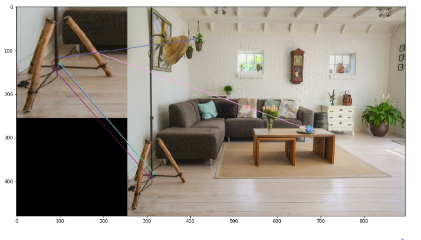
FLann based matcher using OpenCV
'''
Using Flann-based matching on ORB features
'''import numpy as np
import cv2
from matplotlib import pyplot as plt
import imutils

orb = cv2.ORB_create(500)

img1 = cv2.imread("imgs/chapter9/indoor_lamp.jpg", 1);
img1 = cv2.resize(img1, (256, 256));
gray1 = cv2.cvtColor(img1,cv2.COLOR_BGR2GRAY);

img2 = cv2.imread("imgs/chapter9/indoor.jpg", 1);
img2 = cv2.resize(img2, (640, 480));
gray2 = cv2.cvtColor(img2,cv2.COLOR_BGR2GRAY);

# find the keypoints and descriptors with SIFT
kp1, des1 = orb.detectAndCompute(img1,None)
kp2, des2 = orb.detectAndCompute(img2,None)

# FLANN parameters
FLANN_INDEX_LSH = 6
index_params= dict(algorithm = FLANN_INDEX_LSH,
 table_number = 6, # 12
 key_size = 12, # 20
 multi_probe_level = 1) #2
search_params = dict(checks=50) # or pass empty dictionary
flann = cv2.FlannBasedMatcher(index_params,search_params)
matches = flann.knnMatch(des1,des2,k=2)
# Need to draw only good matches, so create a mask
matchesMask = [[0,0] for i in range(len(matches))]
# ratio test as per Lowe's paper
for i,(m,n) in enumerate(matches):
 if m.distance < 0.7*n.distance:
 matchesMask[i]=[1,0]
draw_params = dict(matchColor = (0,255,0),
 singlePointColor = (255,0,0),
 matchesMask = matchesMask,
 flags = cv2.DrawMatchesFlags_DEFAULT)
img3 = cv2.drawMatchesKnn(img1,kp1,img2,kp2,matches,None,**draw_params)

plt.figure(figsize=(15, 15))
plt.imshow(img3[:,:,::-1])
plt.show()

Image Stitching
- Image stitching or photo stitching is the process of combining multiple photographic images with overlapping fields of view to produce a segmented panorama or high-resolution image.

Image Stitching using OpenCV
from matplotlib import pyplot as plt
%matplotlib inline
import cv2
import numpy as np
import argparse
import sys
modes = (cv2.Stitcher_PANORAMA, cv2.Stitcher_SCANS)# read input imagesimgs = [cv2.imread("imgs/chapter9/left.jpeg", 1),cv2.imread("imgs/chapter9/right.jpeg", 1)]stitcher = cv2.Stitcher.create(cv2.Stitcher_PANORAMA)
status, pano = stitcher.stitch(imgs)f = plt.figure(figsize=(15,15))
f.add_subplot(1, 2, 1).set_title('Left Image')
plt.imshow(imgs[0][:,:,::-1])
f.add_subplot(1, 2, 2).set_title('Right Image')
plt.imshow(imgs[1][:,:,::-1])
plt.show()

plt.figure(figsize=(15, 15))
plt.imshow(pano[:,:,::-1])
plt.show()

You can find the complete jupyter notebook on Github.
If you have any questions, you can reach Abhishek and Akash. Feel free to reach out to them.
I am extremely passionate about computer vision and deep learning in general. I am an open-source contributor to Monk Libraries.
You can also see my other writings at:
Akula Hemanth Kumar – Medium
Read writing from Akula Hemanth Kumar on Medium. Computer vision enthusiast. Every day, Akula Hemanth Kumar and…
medium.com

Join thousands of data leaders on the AI newsletter. Join over 80,000 subscribers and keep up to date with the latest developments in AI. From research to projects and ideas. If you are building an AI startup, an AI-related product, or a service, we invite you to consider becoming a sponsor.
Published via Towards AI
Related posts


Popular posts

 for 2021")


Updates

Recent Posts


